4 Introduction to Fourier Restriction
Theorem (Hausdorff-Young inequality).
Assuming that:
Proof.
The inequality is true for ,
and for ,
the inequality is true since we have equality (Plancherel).
For values in between we can interpolate. □
Are there any other
for which
We saw that
was necessary (translations / modulations, Khinchin’s inequality).
Scaling: Plug in
which is -normalised
(). Then
which is
-normalised
().
|
|
|
|
So we need for all :
So we need ,
i.e. .
Classical questions
What is the smallest
constant such that ?
Which functions
satisfy ?
2014:
|
|
Fourier restriction asks which
permit estimates
( is the restricted
frequency set, ).
Example.
(measure
subset of ).
means
|
|
Always:
true for all .
In the second example, only this trivial statement is true (i.e.
is false for all
other values for ).
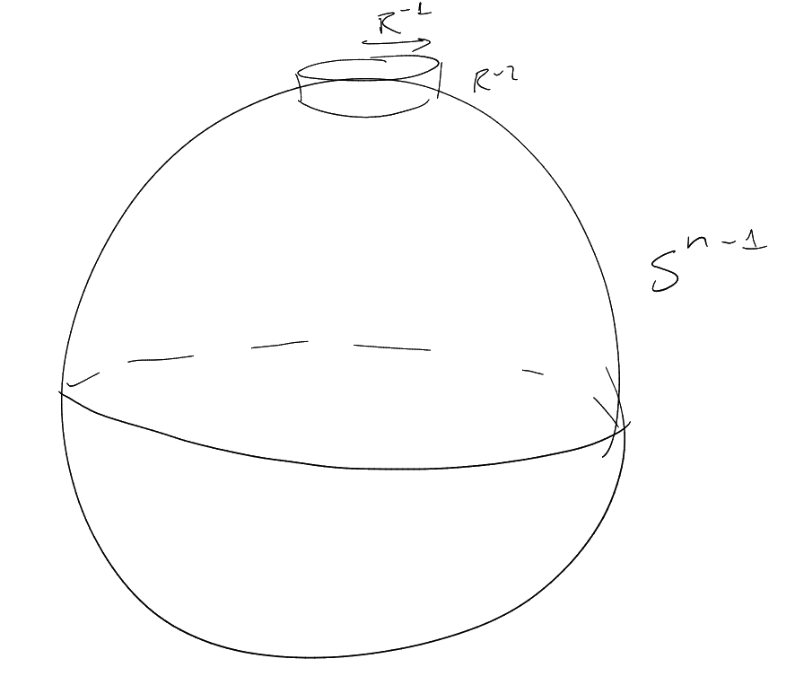
Let be the unit
sphere in .
Consider
where uses the usual
surface measure
on .
Notation.
We may call
the “inverse Fourier transform”.
Let ,
-valued,
on
, with
support in .
May also assume
is -valued,
on
.
bounded,
.
behaves
like in
.
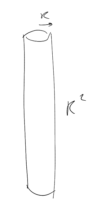
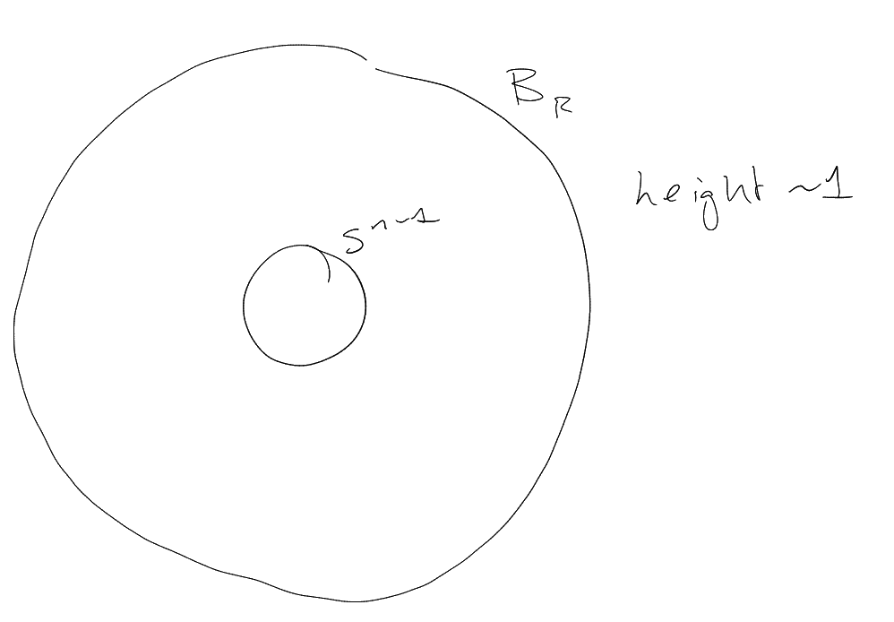
Consider dilates ,
.
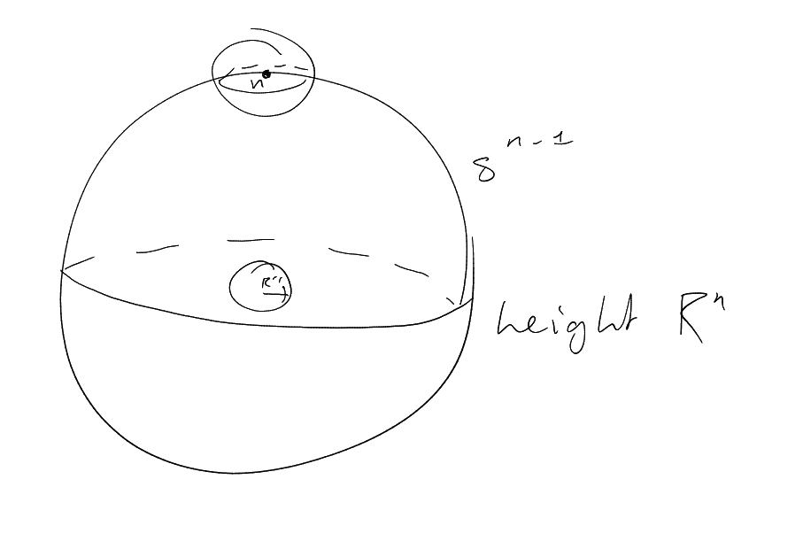
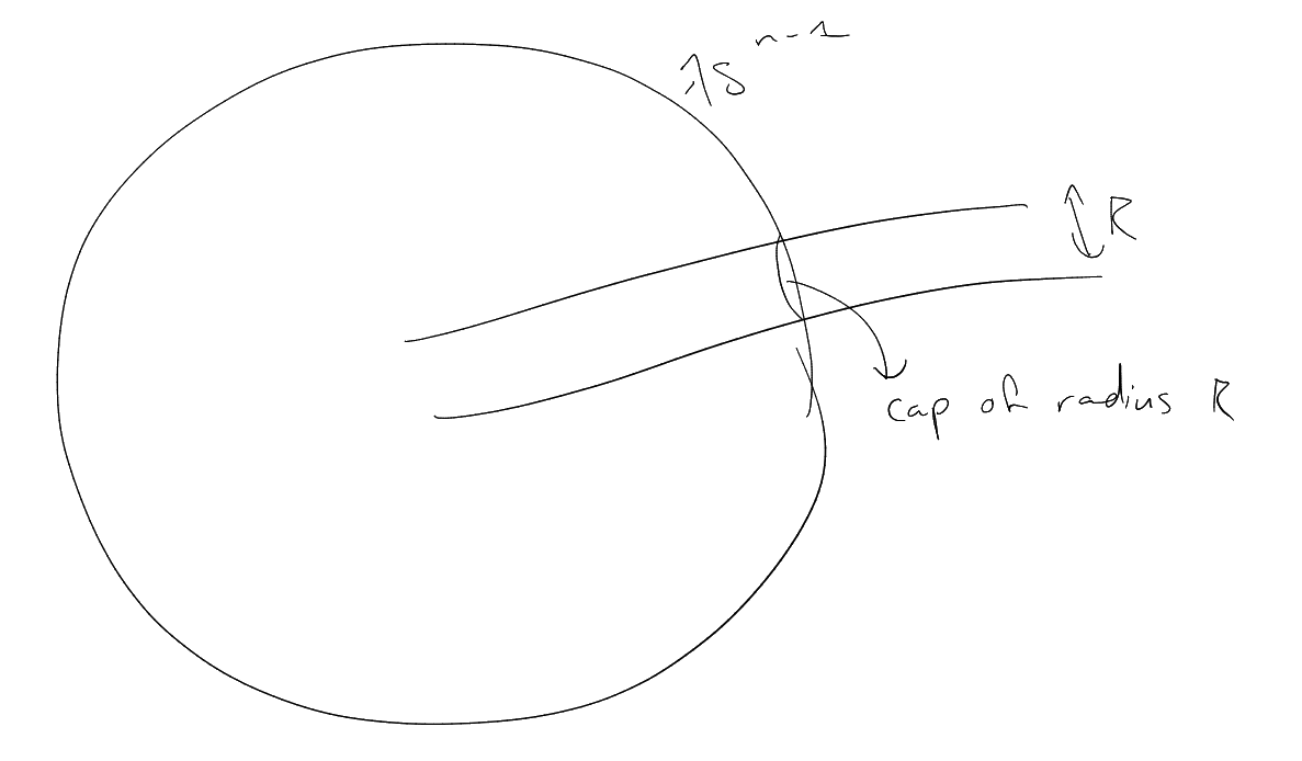
Frequency side
(-norm).
|
|
cap of
radius .
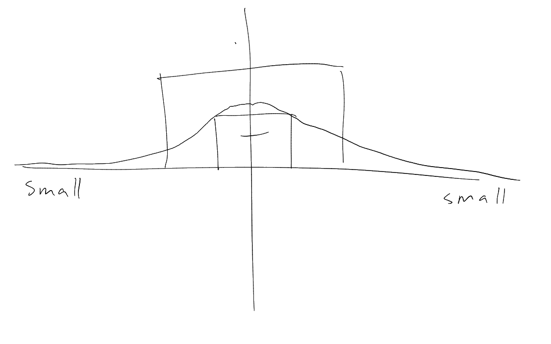
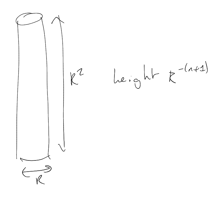
Spacial side
(in -norm).
height ,
.
,
.
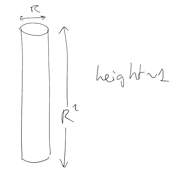
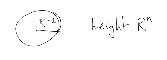
Consider: .
Frequency: .
.
|
|
Spatial side:
(-norm).
.
,
. Implies
B.
On Monday, we will build examples
such that
sees all of .
.
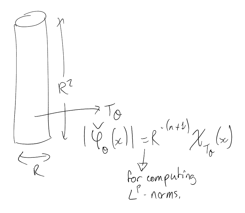
Consider the statement
(recall that we called this ).
Fix ,
. For
computing
norms, .
Wave packet function with localised spatial and frequency behaviour.
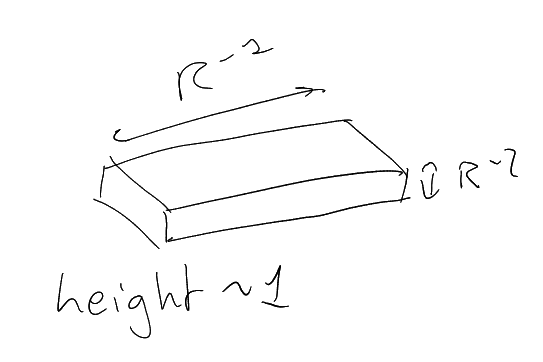
Last time: .
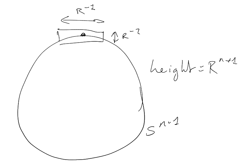
Frequency:
Spatial:
Note: sphere near
looks like ,
.
Naive attempt:
Frequency:
Spatial:
.
Deduce: , so
(trivial).
on
made
easy to
compute.
Could we improve things?
Could think about :
then ,
. This is
more efficient, but we can’t take a limit. So not so useful.
Build a function
which satisfies
on .
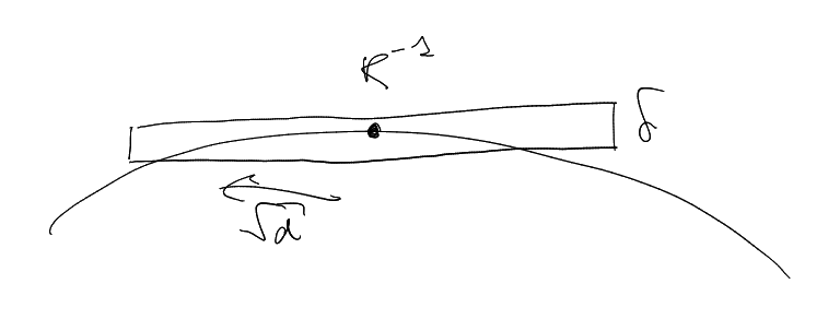
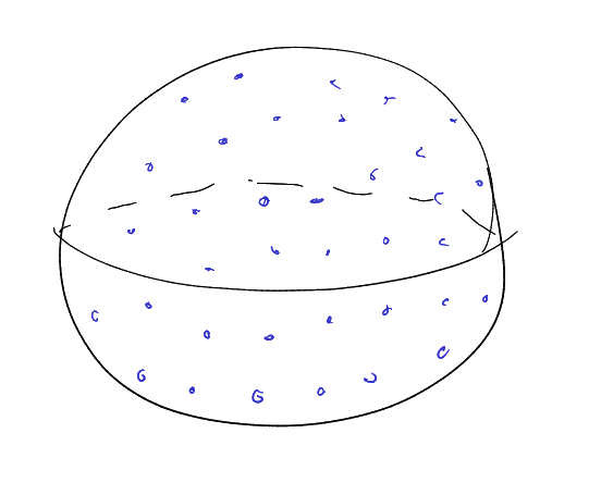
Let be a maximal
collection of -spaced
points on
().
For each ,
let be
an affine map which sends
|
|
Define ,
.
on
(actually on
-neighbourhood
of ).
.
.
Frequency:
Spatial:
.
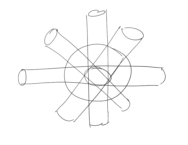
“bush of tubes”
many
tubes in
-separated
directions
|
|
Compute
Consider overlap of
on
().
Average overlap on :
|
|
Not too hard to check that the number of active
on is
.
Now calculate:
|
|
|
|
Two cases: either dominates or
the other term dominates. So .