What is Fourier Restriction Theory?

1 What is Fourier Restriction Theory?

Main object: $f : ℝ^{d} \to ℂ$ , $f (x) = \sum_{ξ \in ℝ} b_{ξ} e^{2 π i x \cdot ξ}$ , $b_{ξ} \in ℂ$ .

Notation. We will write $e (x \cdot ξ) i e^{2 π i x \cdot ξ}$ .

$x \in ℝ^{d}$ is a spatial variable, and $ξ \in ℝ^{d}$ is the frequency variable.

The frequencies (or Fourier transform) of $f$ is restricted to a set $R$ (where $R$ we will always be finite – so no need to worry about convergence issues).

Goal: Understand the behaviour of $f$ in terms of properties of $R$ .

Example.

(i) Schrödinger equation:
Easy: $(2 π i \partial_{+} - Δ) u = 0$ , with initial data $u (x, 0) = \sum_{n - 1}^{N} b_{n} e (n x)$ .
$(x, t) = (x_{1}, x_{2})$ . Then since $e (n x + n^{2} t) i e ((n, n^{2}) \cdot (x, t))$ , we might consider $R = {(n, n^{2}) : n = 1, \dots, N}$ .
(ii) Dirichlet polynomials:
with $b_{n} \equiv 1$ , partial sums of Riemann Zeta function. We might consider $R = {\frac{1}{2 π} \log n}_{n = N}^{2 N}$ .

Both avoid linear structure.

${\log n}$ is a concave set (getting closer and closer together).

${(n, n^{2})}$ lie on a parabola.

Guiding principle: if properties of an object avoid (linear) structure, then we expect some random or average behaviour.

The above examples avoid linear structure using some notion fo curvature. See Bourgain $Λ (p)$ paper: $\to$ extra behaviour.

Square root cancellation: If we add $\pm 1$ randomly $N$ times, then we expect a quantity with size $N^{\frac{1}{2}}$ .

Theorem 1.1 (Khinchin’s inequality). Assuming that:

${𝜀_{n}}_{n = 1}^{N}$ be IID random variables with $ℙ (𝜀_{n} = 1) = ℙ (𝜀_{n} = - 1) = \frac{1}{2}$
$1 < p < \infty$
$x_{1}, \dots, x_{N} \in ℂ$

Then

( ||N∑ ||p) 1p (∑N ) 12
𝔼|| 𝜀nxn|| ∼p |xn|2 = ∥xn∥2.
|n=1 | n=1

Notation. $\sim_{p}$ means $\sim$ but the constant may depend on $p$ .

Proof. Without loss of generality, $x_{1}, \dots, x_{n} \in ℝ$ . Without loss of generality, $∥ x ∥_{2} = 1$ .

$p = 2$ : want to show $𝔼 ({| \sum_{n} 𝜀_{n} x_{n} |}^{2}) \sim 1$ .

( )
∑ ∑------- ∑ --- ∑ 2 ∑ ∑ ---
𝔼 𝜀nxn 𝜀mxm = 𝔼(𝜀n𝜀mxnxm ) = |xn| + xn xm◟𝔼◝𝜀◜n◞𝔼𝜀m.
n m n,m n n m=n =0

What about general exponents

p

( | | ) ( | | )
||∑ ||p ∫ ∞ ||∑ ||p
𝔼 || 𝜀nxn|| = ℙ || 𝜀nxn || > α dα.
n 0 n

The equality here is the Layer cake formula, which is true for any

p \in (0, \infty)

Let $λ > 0$ . Study the random variable $e^{λ \sum_{n} 𝜀_{n} x_{n}} \in (0, \infty)$ .

( ) ( ) ( )
𝔼 eλ∑n 𝜀nxn = 𝔼 ∏ eλ𝜀nxn = ∏ 𝔼eλ𝜀nxn = ∏ 1eλxn + 1e−λxn .
n n n 2 2

Fact:

\frac{1}{2} e^{z} + \frac{1}{2} e^{- z} \leq e^{\frac{z^{2}}{2}}

(to check, use the Taylor series). So we can get

\begin{array}{l} α ℙ (e^{λ \sum_{n} 𝜀_{n} x_{n}} > α) & \leq 𝔼 (e^{λ \sum_{n} 𝜀_{n} x_{n}}) & (Chebyshev’s inequality) \\ \leq \prod_{n} e^{λ^{2} | x_{n} |^{2} ∕ 2} \\ = e^{λ^{2} ∕ 2} \end{array}

By symmetry,

Choose

α = e^{λ^{2}}

(| | ) (| |p )
||∑ || ||∑ || p −λ2∕2
ℙ || 𝜀nxn|| > λ = ℙ || 𝜀nxn|| > λ ≲ e .
n n

Use in Layer cake:

( || ||p) ∫ ∞
𝔼 ||∑ 𝜀 x || ≲ e−α2∕p∕2dα ∼ 1.
| n n n| 0 p

Lower bound: use Hölder’s inequality.

X = \sum_{n} 𝜀_{n} x_{n}

-- p 1∕p q1∕q
𝔼◟(X◝◜X)◞ ≤ (𝔼◟-(|X◝|◜))-◞(𝔼|X | ) .
=1 ≲p1

\frac{1}{p} + \frac{1}{q} = 1

. □

Can you find a more intuitive proof? E-mail Dominique Maldague.

Corollary. $𝔼 (\int {| \sum_{n = 1}^{N} 𝜀_{n} f_{n} (x) |}^{p} d x) \sim_{p} \int {| \sum_{n = 1}^{N} | f_{n} (x) |^{2} |}^{p ∕ 2} d x$ .

Useful for exercises!

Return to Fourier restriction context.

\begin{array}{l} f (x) & = \sum_{n = 1}^{N} e (n x) & R & = {1, \dots, N} \\ g (x) & = \sum_{n = 1}^{N} e (n^{2} x) & R & = {1^{2}, 2^{2}, \dots, N^{2}} \end{array}

Both $f, g$ are $1$ -periodic. So study them on $𝕋 = [0, 1]$ . $f (0) = N$ , $| f (x) | \sim N$ for $\in [0, c \frac{1}{N}]$ . $g (0) i N$ , $| g (x) | \sim N$ for $x \in [0, c \frac{1}{N^{2}}]$ .

∫ ∑ ∫
|f(x)|2dx = e((n− mx )dx = N).
[0,1] n,m [0,1]

∫ ∑ ∫
|g(x )|2 = e((n2 − m2 )x)dx = N.
[0,1] n,m [0,1]

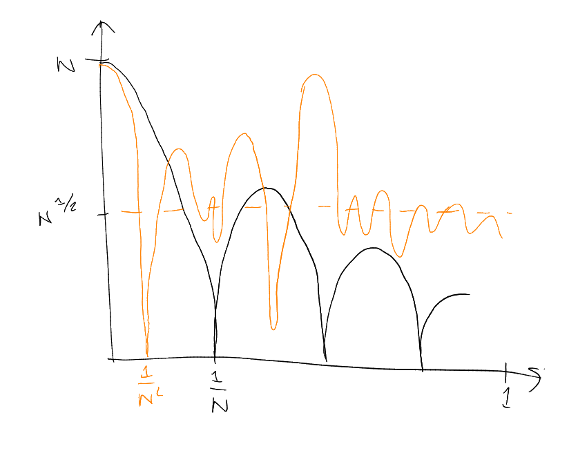
For the first one,

N^{p - 1}

(organised behaviour) dominates as soon as

p > 2

, and for the second one,

N^{p ∕ 2}

dominates for

2 \leq p \leq 4

(“square root cancellation behaviour lasts for longer”).

[next] [prev] [prev-tail] [front] [up]