5 Equivalent Versions of Fourier Restriction

Searching for $(p,q)$ for which

• (1)

  

  $R={[0,1]}^{n-1}\times \{0\}$

  

• (2)

  

  $\to {\int }_{B_{R^2}}{\left|{\sum }_{𝜃}{\chi }_{T_{𝜃}}\right|}^{\frac{p}{2}}$. “continuum incidence geometry problem”.

  

  integral equals $={\sum }_{B_R\subseteq B_{R^2}}{\int }_{B_R}{\left|{\sum }_{𝜃}{\chi }_{T_{𝜃}}\right|}^{\frac{p}{2}}$.

  “fractal geometry”.

  

Reminder: $R_{S^{n-1}}(p\to q)$ means

First proved for $S^1\subseteq {ℝ}^2$ by Fefferman (1970) and Zygmund (1974).

Special things happen in ${ℝ}^2$, classical harmonic analysis techniques apply.

Same conjecture for $R_{P^{n-1}}(p\to q)$, where

For $n\ge 3$, open and active!

Restriction theory can be used to deduce continuum incidence geometry estimates.

Surprisingly, we can go the other way too (very recent progress, whereas the above direction has been well-known since at least the $90$s).

Equivalent formulations of $R_{P^{n-1}}(p\to q)$

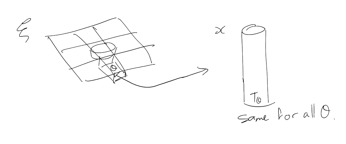
Dual version is called “Fourier extension”:

Call the last inequality $R_{P^{n-1}}^{\ast }(q^{\prime }\to p^{\prime })$.

Local, dual version: allows us to work with functions, F.T.

For any $R\ge 1$, any $B_R\subseteq {ℝ}^n$, we have

Call this $R_{P^{n-1}}^{\ast ,\text{loc}}(q^{\prime }\to p^{\prime })$.

$R_{P^{n-1}}^{\ast }(q^{\prime }\to p^{\prime })⟹R_{p^{n-1}}^{\ast ,\text{loc}}(q^{\prime }\to p^{\prime })$. First thing bounds $Eg$, while secound thing bounds $f$ when we have $\mathrm{supp}\widehat{f}\subseteq N_{R^{-1}}(P^{n-1})$.

Let $f\in S({ℝ}^n)$, $\mathrm{supp}\widehat{f}\subseteq N_{R^{-1}}(P^{n-1})$. Try to express $f$ in trems of ext. op.

using RPn−1∗(q′→ p′) Goal is to bound this last expression by

Lucy case: $\frac{p^{\prime }}{q^{\prime }}<1$, i.e. $1<\frac{q^{\prime }}{p^{\prime }}$. Then

$s\ge 1$ (actually $\approx$ since $h$ approximately constant on $A$)

$R_{P^{n-1}}^{\ast }(q^{\prime }\to p^{\prime })⟹R_{P^{n-1}}^{\ast ,\text{loc}}(q^{\prime }\to p^{\prime })$ continued.

Spatial: $x,f(x),Eg(x)$

Frequency $\xi$:

$g({\xi }^{\prime },|{\xi }^{\prime }{|}^2)=g({\xi }^{\prime })$, $\mathrm{supp}\widehat{f}\subseteq N_{R^{-1}}(P^{n-1})$,

Aiming for

Lucky case: $\frac{p^{\prime }}{q^{\prime }}\le 1$.

$R^{-(p^{\prime }-1)}{(R^{-1})}^{1-\frac{p^{\prime }}{q^{\prime }}}=R^{-\frac{p^{\prime }}{q}}$ ($1=\frac{1}{q}+\frac{1}{q^{\prime }}$)

Unlucky case: $\frac{p^{\prime }}{q^{\prime }}>1$. Hölder’s inequality goes in the wrong direction:

for all $s\ge 1$, $h\ge 0$.

This is equality if $h$ is constant on $A$.

PAUSE THIS.

Useful Harmonic Analysis tool

The locally constant property.

Convolution: Let $f,g\in S({ℝ}^n)$. Define $f\ast g\in S({ℝ}^n)$ by

See Young’s convolution:

when $1+\frac{1}{r}=\frac{1}{p}+\frac{1}{q}$.

Example. $g={\chi }_B$ ($B$ is the unit ball in ${ℝ}^n$),

RHS is “average value of $f$ on $B(x)$”.

“$f\ast {\chi }_B$ is approximately constant on balls of radius $\sim 1$”.

Support property: $\mathrm{supp}f=A$, $\mathrm{supp}g=B$, $\mathrm{supp}f\ast g\subseteq A+B=\{a+b:a\in A,b\in B\}$.

Convolution and Fourier Transform: $\widehat{fg}=\widehat{f}\ast \widehat{g}$.

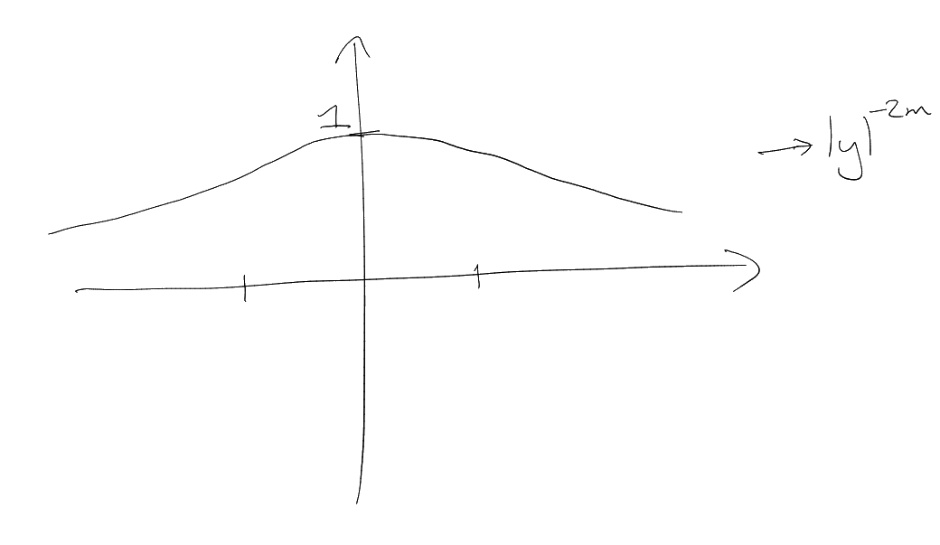
Locally constant property: Let $f\in S({ℝ}^n)$, $\mathrm{supp}\widehat{f}\subseteq B_1(0)$. Then for any unit ball $B^{\prime }\subseteq {ℝ}^n$ and any $x\in B^{\prime }$,

$\frac{1}{{(1+|y{|}^2)}^m}$ is $\sim 1$ on $|y|\lesssim 1$.

Digesting $f\ge 0$.

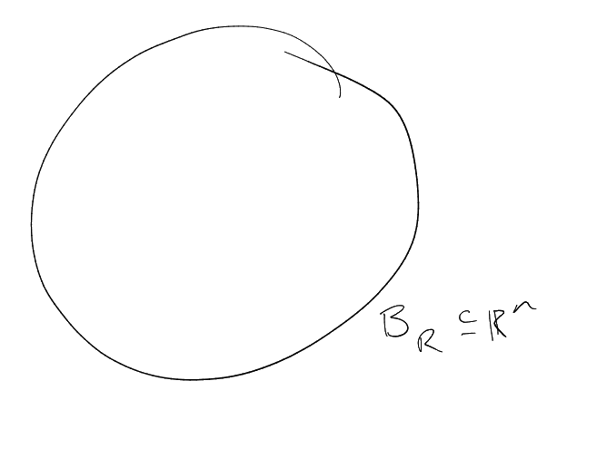
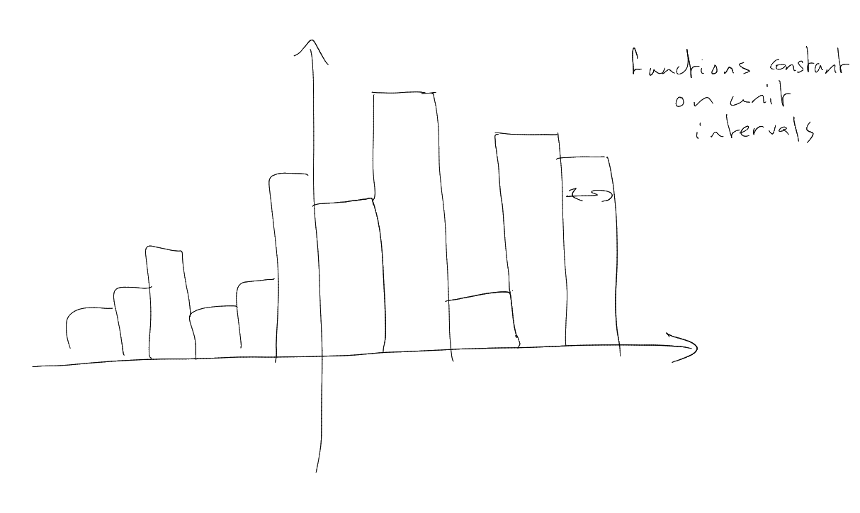
For any unit interval $I^{\prime }\subseteq {ℝ}^n$, $x\in I^{\prime }$,

Suppose this:

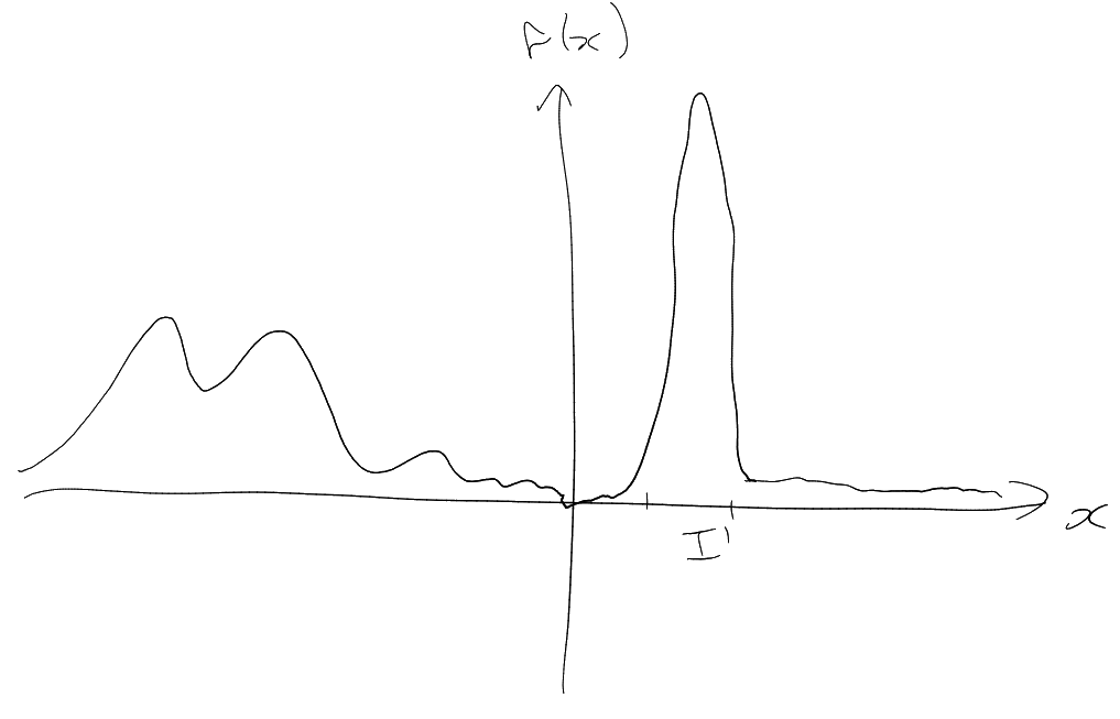
LHS has to be constant.

Lemma (Locally constant property). Assuming that:

• $f\in S({ℝ}^n)$

• $\mathrm{supp}\widehat{f}\subseteq B_1(0)$

Then for any unit ball $B^1\subseteq {ℝ}^n$ and any $x\in B^{\prime }$,

The proof of this fact is more important than the statement – we will be using the strategy in future.

Proof of locally constant property. Let $f\in S({ℝ}^n)$, $\mathrm{supp}\widehat{f}\subseteq B_1(0)$. Let $\phi \in C_c^{\infty }({ℝ}^n)$ such that $\phi \equiv 1$ on $B_1(0)$, $\mathrm{supp}\phi \subseteq B_2(0)$.

By Fourier inversion:

Let $x_0,x\in B^1$ (unit ball in ${ℝ}^n$).

Returning to $R_{P^{n-1}}^{\ast }(q^{\prime }\to p^{\prime })⟹R_{P^{n-1}}^{\ast ,\text{loc}}(q^{\prime }\to p^{\prime })$

where ${\phi }_{B_R}\in S({ℝ}^n)$ satisfies ${\phi }_{B_R}\sim 1$ on $B_R$, $\mathrm{supp}\widehat{{\phi }_{B_R}}\subseteq B_{R^{-1}}(0)$.

supported in $2R^{-1}$-neighbourhood of $P^{n-1}$.

Repeat steps of proof:

$$\begin{array}{llll}\hfill {\int }_{B_R}|f(x){|}^{p^{\prime }}dx& \lesssim R^{-(p^{\prime }-1)}{\int }_{I_{R^{-1}}}{\left({\int }_{|{\xi }^{\prime }|<1}|h_{{\xi }_n}({\xi }^{\prime }){|}^{q^{\prime }}d{\xi }^{\prime }\right)}^{\frac{p^{\prime }}{q^{\prime }}}d{\xi }_n& \hfill & \end{array}$$

[next] [prev] [prev-tail] [front] [up]