Exponential sums in Lp

2 Exponential sums in $L^{p}$

Recall: studying $f (x) = \sum_{ξ \in R} e (ξ \cdot x)$ . When $R$ does not have (linear) structure, expect $| f (x) | \sim | R |^{\frac{1}{2}}$ (“sqrt cancellation”) in an appropriate sense (in $L^{p}$ ), more than when $R$ is structured.

Linear $R$ $f (x) = \sum_{n = 1}^{N} e (n x)$ vs convex $R$ $g (x) = \sum_{n = 1}^{N} e (n^{2} x)$ .

Have

∫ ∫
|f(x)|2dx = N = |g(x)|2dx.
[0,1] [0,1]

Have

| f (x) | \sim N

[0, c N^{- 1}]

, and

| g (x) | \sim N

[0, c N^{- 2}]

$L^{2}$ does not distinguish $f, g$ . $L^{\infty}$ does not distinguish. However, $2 < p < \infty$ does.

What about $1 \leq p \leq 2$ ? We don’t usually study this range because the estimates tend to be trivial / not interesting.

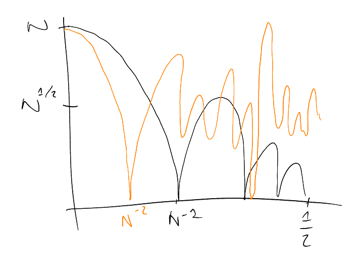
Focus on $2 < p < \infty$ . Preduct size of

Square root cancellation lower bound:

∫ ( ∫ ) 2p
N = |f |2 H öl≤der’s |f|2⋅p2 (1)□
[0,1] [0,1]

⟹ N^{p ∕ 2} \leq \int_{[0, 1]} | f |^{p}

Constant integral lower bound:

\begin{array}{l} \int_{[0, 1]} | f |^{p} & \geq \int_{[0, c N^{- 1}]} | f |^{p} ≳ N^{p} N^{- 1} \\ \int_{[0, 1]} | g |^{p} & \geq \int_{[0, c N^{- 2}]} | g |^{p} ≳ N^{p} N^{- 2} \end{array}

$\int | f |^{p} ≲ N^{p ∕ 2} + N^{p - 1}$ , $\int | g |^{p} ≲ N^{p ∕ 2} + N^{p - 2}$ .

Note that for the $f$ bound, $N^{p - 1}$ is bigger than $N^{p - 1}$ (as long as $p > 2$ ), so the constant integral dominates!

For $g$ , if $2 \leq p \leq 4$ , the square root cancellation dominates, but for $p > 4$ the constant integral takes over.

Assuming:

Theorem 2.1. - $p > 2$ - $b_{n} \in ℂ$ Then:

∫ ||∑ ||p
|| bne(nx)|| ≤ N p2−1∥bn∥p2.
| n |

Proof. Consider: $\sum_{n = 1}^{N} b_{n} e (n x)$ , $b_{n} \in ℂ$ .

\begin{array}{l} \int_{[0, 1]} {| \sum_{n} b_{n} e (n x) |}^{p} d x & \leq {∥ \sum_{n} b_{n} e (n x) ∥}_{\infty}^{p - 2} \int_{[0, 1]} {| \sum_{n} b_{n} e (n x) |}^{2} d x \\ \leq {(N^{\frac{1}{2}} ∥ b_{n} ∥_{2})}^{p - 2} ∥ b_{n} ∥_{2}^{2} & CS \\ = N^{\frac{p}{2} - 1} ∥ b_{n} ∥_{2}^{p} □ \end{array}

Note that this is sharp when $b_{n} \equiv 1$ .

$\sum_{n = 1}^{N} b_{n} e (n^{2} x)$ . Focus on $p = 4$ .

| |4
∫ ||∑ 2 || ∑ ∑ ∑ ∑ ------∫ 2 2 2 2
[0,1]|| bne(n x)|| dx = bn1bn2bn3bn4 [0,1]e((n1 + n2 − n3 − n4)x)dx.
n n1 n2 n3 n4

The integral vanishes unless

n_{1}^{2} - n_{3}^{2} = n_{4}^{2} - n_{2}^{2}

Number Theory lemma: If $m \in ℤ$ , then

Follows from unique prime factorisation.

Warning. The above lemma is false.

See correction later.

For fixed $n_{1}, n_{3}$ ,

2 2
# {◟(n2,n4) : n1 −-n3-=◝◜(n4 +-n2)(n4-−-n2)}◞≲ log N.
=:𝒮n1,n3

Hence

\begin{array}{l} \int_{[0, 1]} {| \sum_{n} b_{n} e (n^{2} x) |}^{4} d x & \leq \sum_{n_{1}} \sum_{n_{3}} | b_{n_{1}} b_{n_{3}} | | \sum_{(n_{2}, n_{4}) \in S_{n_{1}, n_{3}}} b_{n_{2}} b_{n_{4}} | \\ ≲ (\log N) ∥ b_{n} ∥_{2}^{4} \end{array}

We will now use $≾$ to mean $≲$ up to powers of $\log N$ .

$2 < p < 4$ : $\frac{1}{p} = \frac{𝜃}{2} + \frac{1 - 𝜃}{4}$ , $𝜃 \in [0, 1]$ , $h = \sum_{n} b_{n} e (n^{2} x)$ , $∥ h ∥_{p} \leq ∥ h ∥_{2}^{𝜃} ∥ h ∥_{4}^{1 - 𝜃} ≾ ∥ b_{n} ∥_{2}^{𝜃} ∥ b_{n} ∥_{2}^{1 - 𝜃} \approx ∥ b_{n} ∥_{2}$ .

$p \geq 4$ :

∫
p p− 4 4 CS 12 p−4 4 p2−2 p
[0,1]|h| ≾ ∥h∥∞ ∥bn∥2 ≤ (N ∥bn∥2) ∥bn∥2 ≈ N ∥bn∥2.

Assuming:

Theorem 2.2. - $2 > p$ Then:

∫ ||∑ ||p
|| bne(n2x)|| dx ≾ (1 = N p2− 2)∥bn∥p2.
|n |

Sharp by $b_{n} \equiv 1$ .

Positive take away: estimates are sharp, proofs are elementary. Easy to think of sharp examples.

Number Theory counting idea shows:

\begin{array}{l} \int_{{[0, 1]}^{2}} | u (x, t) |^{6} d x d t & ≾ ∥ b_{n} ∥_{2}^{6} & u (x, t) & = \sum_{\begin{array}{c} | n | \sim N \\ n \in ℤ \end{array}} b_{n} e (n x + n^{2} t) \\ \int_{{[0, 1]}^{3}} | u (x, t) |^{4} d x d t ≾ ∥ b_{n} ∥_{2}^{4} & u (x, t) & = \sum_{\begin{array}{c} | n | \sim N \\ n \in ℤ^{2} \end{array}} b_{n} e (n \cdot x + | n |^{2} t) \end{array}

Sharp, $6, 4 = p_{crit}$ .

Strichartz estimate for periodic Schrödinger equation, observed by Bourgain in 1990s.

Negatives: on $𝕋^{3}$ $\to$ $p_{crit} = \frac{10}{3}$ , but this technique can only work on even integer values of $p$ .

$𝕋^{1}$ , $𝕋^{2}$ only sharp Strichartz estimates per Schrödinger until 2015!

2015: Bourgain-Demeter proved $(l^{2}, L^{p})$ sharp decoupling estimate. Gives sharp Strichartz estimate for Schrödinger in $𝕋^{d}$ for all $d$ .

Proved earlier:

| |
∫ ||∑ ( n2 )||p p p
N −2 2 || e N-2x || dx ≤ (1+ N 2−2)∥bn ∥2.
[0,N ] n∼N

(where

n \sim N

means

N \leq n \leq 2 N

Conjecture:

∫ | |p
− ||∑ b e(a x)|| dx ≲ (1 + N p2−2)∥b ∥p
[0,N2]||n∈N n n || n 2

$a_{n} \in [0, 1]$ , $a_{n + 1} - a_{n} \sim \frac{1}{N}$ , $a_{n + 2} - a_{n + 1} - (a_{n + 1} - a_{n}) \sim \frac{1}{N^{2}}$ .

Example: ${a_{n}} \sim {\frac{n^{3}}{N^{3}}}_{n = N}^{2 N}$ .

[next] [prev] [prev-tail] [front] [up]

2 Exponential sums in Lp

2 Exponential sums in $L^{p}$