Dependent Random Choice - Probabilistic Combinatorics

6 Dependent Random Choice

Definition 6.1 ( $(s, k)$ -rich). Let $G$ be a graph. Say that $R \subset V (G)$ is $(s, k)$ -rich if for every $x_{1}, \dots, x_{s} \in R$ we have

| N (x_{1}) \cap \dots \cap N (x_{s}) | \geq k .

Theorem 6.2 (Dependent Random Choice). Assuming that:

$G$ a graph on $n$ vertices with $e (G) = m$
$s, t, r, k \geq 0$
$\frac{{(2 m)}^{t}}{n^{2 t - 1}} - (\binom{n}{s}) {(\frac{k}{n})}^{t} \geq r$

Then there exists

R \subset V (G)

| R | \geq r

which is

(s, k)

-rich.

Note that $t$ doesn’t appear in the conclusion. It is a parameter that we can tune appropriately in applications.

Proof. We sample $x_{1}, \dots, x_{t} \in V (G)$ uniformly at random (with replacement). Then

\begin{array}{l} 𝔼_{x_{1}, \dots, x_{t}} | N (x_{1}) \cap \dots \cap N (x_{t}) | & = 𝔼_{x_{1}, \dots, x_{t}} \sum_{y \in V (G)} 𝟙_{x_{1} \sim y \land x_{2} \sim y \land \dots \land x_{t} \sim y} \\ = \sum_{y \in V (G)} {[ℙ_{x_{1}} (x_{1} \sim y)]}^{t} \\ = \sum_{y \in V (G)} {(\frac{d (y)}{n})}^{t} \\ \geq n {(\frac{2 m}{n^{2}})}^{t} \\ = \frac{{(2 m)}^{t}}{n^{2 t - 1}} \end{array}

Let $Y$ be the random variable that counts the number of ${y_{1}, \dots, y_{s}} \in {(N (x_{1}) \cap \dots \cap N (x_{t}))}^{(s)}$ with

| N (y_{1}) \cap \dots \cap N (y_{s}) | < k .

We want $Y$ to be not too big. This will be the case (on average) because $ℙ (y_{1}, \dots, y_{s} \in N (x_{1}) \cap \dots \cap N (x_{t}))$ is an increasing function of $| N (y_{1}) \cap \dots \cap N (y_{s}) |$ (so our probability distribution is biased away from fully selecting tuples that will increase $Y$ ). We make this precise as follows:

Note

Y = \sum_{\begin{array}{c} {y_{1}, \dots, y_{s}} \in {(V (G))}^{(s)} \\ | N (y_{1}) \cap \dots \cap N (y_{s}) | < k \end{array}} 𝟙_{y_{1}, \dots, y_{s} \in N (x_{1}) \cap \dots \cap N (x_{t})},

\begin{array}{l} 𝔼 Y & \leq \sum_{\begin{array}{c} {y_{1}, \dots, y_{s}} \in {(V (G))}^{(s)} \\ | N (y_{1}) \cap \dots \cap N (y_{s}) | < k \end{array}} ℙ (x_{1}, \dots, x_{t} \in N (y_{1}) \cap \dots \cap N (y_{s})) \\ \leq (\binom{n}{s}) {(\frac{k}{n})}^{t} \end{array}

To finish, define $R$ to be $N (x_{1}) \cap \dots \cap N (x_{t})$ with a vertex deleted from each ${y_{1}, \dots, y_{s}} \in {(⋂_{i = 1}^{t} N (x_{i}))}^{(s)}$ with $| N (y_{1}) \cap \dots \cap N (y_{s}) | < k$ . By definition, $R$ is $(s, k)$ -rich, so we now just need to ensure that $| R | \geq r$ holds for some choice of $x_{1}, \dots, x_{t}$ . Indeed,

\begin{array}{l} | R | & \geq | N (x_{1}) \cap \dots \cap N (x_{t}) | - Y (x_{1}, \dots, x_{t}) \\ 𝔼 | R | & \geq \frac{{(2 m)}^{t}}{n^{2 t - 1}} - (\binom{n}{s}) {(\frac{k}{n})}^{t} \\ \geq r \end{array}

The last line follows from the assumption. □

Definition 6.3 (Extremal number). Let $H$ be a graph. The extremal numbers of $H$ are

ex (n, H) = \max {e (G) : G ⁄ \supset H, G on n vertices} .

Theorem 6.4 (Erdős-Stone). Assuming that:

$H$ a graph
$χ (H) = r \geq 3$

Then

ex (n, H) = (1 - \frac{1}{r - 1} + o (1)) (\binom{n}{2}) .

Definition 6.5 (Complete bipartite graph). $K_{s, t}$ is the complete bipartite graph with parts of sizes $s$ , $t$ respectively.

If $χ (H) \geq 3$ , then for all $s, t$ , we have $K_{s, t} ⁄ \supset H$ . More generally, a complete $(χ (H) - 1)$ -partite graph will not contain a copy of $H$ . Erdős-Stone says that these constructions are optimal, up to $o (1) (\binom{n}{2})$ edges.

Erdős-Stone doesn’t help us when $χ (H) = 2$ . In this case, it is true that

c n^{2 - \frac{1}{2 t}} \leq ex (n, K_{t, t}) \leq C_{t} n^{2 - \frac{1}{t}} .

See Part II Graph Theory for proofs of both bounds.

These bounds are essentially the best known for $t \geq 5$ .

We now prove a generalisation of this upper bound that holds for graphs other than complete bipartite graphs:

Theorem 6.6 (Füredi). Assuming that:

$H$ be a bipartite graph with vertex partition $A \cup B$
$\deg (x) \leq s$ for all $x \in B$

Then

ex (n, H) \leq C_{H} n^{2 - \frac{1}{s}},

for some $C_{H} > 0$ ( $C_{H}$ depends only on $H$ and not on $n$ ).

Lemma 6.7. Assuming that:

$H$ be a bipartite graph with vertex partition $A \cup B$
$\deg (x) \leq s$ for all $x \in B$
$G$ a graph
$R \subset V (G)$ a $(s, | V (H) |)$ -rich set
$| R | \geq | A |$

Then

G \supset H

Proof. First inject $A \to R$ . We now inductively place the vertices $B = {y_{1}, \dots, y_{l}}$ . Assume we have embedded $y_{1}, \dots, y_{i}$ into $G$ . To embed $y_{i + 1}$ , simply consider the $N (y_{i + 1})$ . These have been embedded inside of $R$ and thus have $\geq | V (H) |$ common neighbours. So there must be a choice for $y_{i + 1}$ that does not clash with the previous choices. □

Proof of Füredi. We are given $G$ with $e (G) \geq C n^{2 - \frac{1}{s}}$ . We choose $C = 2 | H |$ , and will show $G \supset H$ . By lemma, enough to find a $(s, | V (H) |)$ -rich set of size $\geq | A |$ . Let $h = | V (H) |$ and $t = s$ . Then

\begin{array}{l} \frac{{(2 C n^{2 - \frac{1}{s}})}^{t}}{n^{2 t - 1}} - (\binom{n}{s}) {(\frac{h}{n})}^{t} & \geq {(2 C)}^{s} - n^{s} {(\frac{h}{n})}^{s} \\ = {(4 h)}^{s} - h^{s} \\ \geq h \\ \geq | A | \end{array}

as desired. □

Definition 6.8 (Hypercube graph). $Q_{d}$ denotes the hypercube graph: the graph with $V (Q_{d}) = {0, 1}^{d}$ and $x, y \in {0, 1}^{d}$ are adjacent if they differ in exactly one coordinate.

Theorem 6.9. $R (Q_{d}) \leq 2^{10 d}$ .

Proof. Let $n = 2^{10 d}$ and let $χ$ be a colouring of $K_{n}$ . Let $G$ be the graph of the majority colour. So $e (G) \geq \frac{1}{2} (\binom{n}{2}) \geq \frac{n^{2}}{8}$ . So we apply Dependent Random Choice to find a $(d, 2^{d})$ -rich set of size $\geq 2^{d}$ . If $t = 2 d$ , then

\begin{array}{l} \frac{{(n^{2} ∕ 4)}^{t}}{n^{2 t - 1}} - {(\frac{e n}{d})}^{d} \cdot {(\frac{2^{d}}{n})}^{t} & \geq \frac{n}{4^{2 d}} - n^{d} \frac{2^{d \cdot t}}{n^{2 d}} \\ \geq \frac{n}{4^{2 d}} - \frac{2^{2 d^{2}}}{2^{10 d^{2}}} \\ \geq 2^{d} \end{array}

Then finish by applying Lemma 6.7.

The reasoning for choosing $t = 2 d$ is that we wanted to make ${(\frac{2^{d}}{n})}^{t}$ win against the ${(\frac{e n}{d})}^{d}$ . Setting $t = d$ makes the powers of $n$ cancel, but then we are still left with the big $2^{d t}$ term, so instead we make $t$ a bit bigger than $d$ . □

Remark. One can use this proof to get

R (Q_{d}) \leq 2^{3 d} .

Burr-Erdős conjectured that $R (Q_{d}) \leq C 2^{d}$ . State of the art: $R (Q_{d}) \leq 2^{(2 - 𝜀) d}$ by Tikhomirov 2023.

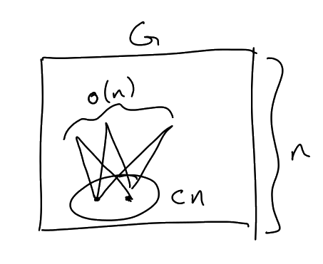
Say I have a graph $H$ , with max degree $d$ where $d$ fixed and $| V (H) | = k \to \infty$ . Then it is known that

R (H) \leq C_{d} \cdot k . (∗)

Proposition 6.10. Assuming that:

$d \geq 1$ , $𝜀 > 0$
$k \geq k_{0}$ , for some $k_{0}$ depending on $d$ and $𝜀$
$H$ bipartite and max degree $\leq d$

Then

R (H) \leq k^{1 + 𝜀} .

Proof. Apply Dependent Random Choice and embedding Lemma 6.7 to the majority colour. □

So Dependent Random Choice and Lemma 6.7 are enough to prove an upper bound that is almost linear in $k$ , but not quite powerful enough to prove the linear bound as in ( $*$ ).

Remark. To improve this to get the bound $R (H) \leq C_{d} n$ , one idea might be to find a $(d, k)$ -rich set where $k = Θ (n)$ ( $n = C_{d} k$ ), where the rich set has size $Θ (n)$ on $n$ vertices. But this is impossible.

Proposition 6.11. For all $c > 0$ , there exists a graph $G$ with $(\frac{1}{2} + o (1)) (\binom{n}{2})$ edges so that every set of size $\geq c n$ contains some $x, y$ with $o (n)$ common neighbours.

Proof. We won’t prove. □

So we have to go back into the guts of the embedding idea. In some sense, the embedding algorithm was a little bit wasteful: for example, we dumped $A$ into the rich set without any clever choice.

The key idea to improve the previous bound will be to perform a more clever embedding algorithm that requires a weaker notion of rich set. We want to use a weaker notion of rich set so that we can find large linear size rich sets.

Definition 6.12 (Approximately $(s, k)$ -rich). Let $G$ be a graph. Say $U \subset V (G)$ is approximately $(s, k)$ -rich if

| {(x_{1}, \dots, x_{s}) \in U^{s} : d (x_{1}, \dots, x_{s}) < k} | \leq {(\frac{1}{2 s})}^{s} | U |^{s} .

Here we use the notation

d (x_{1}, \dots, x_{s}) = | N (x_{1}) \cap \dots \cap N (x_{s}) | .

Lemma 6.13. Assuming that:

$G$ a graph
$U \subset V (G)$ is approximately $(k, k)$ -rich
$| U | > 2 k$
$H$ a bipartite graph on $k$ vertices with max degree $\leq s$

Then

G \supset H

Lemma 6.14. Assuming that:

$𝜀 > 0$
$G$ a graph with $\frac{𝜀 n^{2}}{2}$ edges on $n$ vertices
$n \geq 4 s 𝜀^{- s} k$

Then there exists

U \subset V (G)

that is approximately

(s, k)

-rich and

| U | > 2 k

Theorem 6.15 (Fox, Sudakov, Conlon). Assuming that:

$H$ a bipartite graph on $k$ vertices
max degree $\leq d$

Then

R (H) \leq C d 2^{d} \cdot k .

Remark. This also improves our bound on $Q_{d}$ :

R (Q_{d}) \leq C d 2^{2 d} .

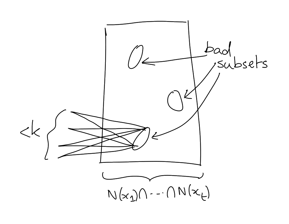
The key difference in proving Lemma 6.13 compared to the previous embedding algorithm is that we will need to embed $A$ in a more clever way. We will need to ensure that for all $b \in B$ , the neighbourhood of $b$ is not sent to one of the bad subsets of $U$ (the “bad” subsets are those which have $< k$ common neighbours).

Proof of Lemma 6.13. For $x_{1}, \dots, x_{t}$ , $t < s$ , let

β (x_{1}, \dots, x_{t}) = | {(x_{1}, \dots, x_{t}, x_{t + 1}, \dots, x_{s}) \in U^{s} : d (x_{1}, \dots, x_{s}) < k} | .

Say that $(x_{1}, \dots, x_{t})$ is healthy if

β (x_{1}, \dots, x_{t}) \leq {(\frac{1}{2 s})}^{s - t} | U |^{s - t} .

We will embed vertices of $A$ one after the other. We will use this notion of healthiness to make sure that every time we place a vertex, we keep plenty of good extensions.

Observation: If $x_{1}, \dots, x_{t}$ is healthy, then the number of $y$ such that $(x_{1}, \dots, x_{t}, y)$ is not healthy is $\leq \frac{| U |}{2 s}$ .

Proof of observation: Note

β (x_{1}, \dots, x_{t}) = \sum_{y \in U} β (x_{1}, \dots, x_{t}, y) .

Let $B_{x_{1}, \dots, x_{t}} = {y : (x_{1}, \dots, x_{t}, y) is not healthy}$ . Then

\begin{array}{l} β (x_{1}, \dots, x_{t}) & \geq \sum_{y \in B_{x_{1}, \dots, x_{t}}} β (x_{1}, \dots, x_{t}, y) \\ \geq | B_{x_{1}, \dots, x_{t}} | {(\frac{1}{2 s})}^{s - t - 1} | U |^{s - t - 1} \end{array}

But if $| B_{x_{1}, \dots, x_{t}} | > \frac{| U |}{2 s}$ , I contradict that $x_{1}, \dots, x_{t}$ is healthy. So we have proved the observation.

We now inject $f : A \to U$ inductively. Assume we have embedded $a_{1}, \dots, a_{i}$ so far. We assume that we have

f (N (b) \cap {a_{1}, \dots, a_{i}})

is healthy for all $b \in B$ . We now embed $a_{i + 1}$ . Let $b_{1}, \dots, b_{s}$ be the neighbour of $a_{i + 1}$ . We know $f (N (b_{i}) \cap {a_{1}, . ., a_{i}})$ are healthy, so there are at most (by observation) $\leq \frac{| U |}{2 s}$ ways of choosing $f (a_{i + 1}) \in U$ so that one of the neighbours becomes unhealthy. But there are only $\leq s$ neighbourhoods. So there are $> \frac{| U |}{2}$ choices that maintain all healthy neighbours. Since $| U | > 2 k$ , I can map $a_{i + 1}$ to a new vertex.

We now inject $f : B \to V (G)$ exactly as we saw in the proof of Lemma 6.7. □

Proof of Lemma 6.14. Let $x_{1}, \dots, x_{s} \in V (G)$ be chosen uniformly at random. Let $U = N (x_{1}) \cap \dots \cap N (x_{s})$ . Let $X = | U |$ . We have $𝔼 X \geq 𝜀^{s} \cdot n$ .

Let $Y = | {(y_{1}, \dots, y_{s}) \in U^{s} : d (y_{1}, \dots, y_{s}) < k} |$ . $𝔼 Y \leq n^{s} {(\frac{k}{n})}^{s}$ . Now note that by Jensen,

𝔼 [X^{s} - \frac{{(𝔼 X)}^{s} Y}{2 𝔼 Y} - \frac{{(𝔼 X)}^{s}}{2}] = 𝔼 X^{s} - {(𝔼 X)}^{s} \geq 0 .

So there is a $U$ such that

| U |^{s} \geq \frac{{(𝔼 X)}^{s}}{2} \geq \frac{{(𝜀^{s} n)}^{s}}{2} .

So $| U | \geq \frac{𝜀^{s} n}{2} > 2 k$ .

Y \leq \frac{2 (𝔼 Y)}{{(𝔼 X)}^{s}} | U |^{s} \leq {(\frac{1}{2 s})}^{s} | U |^{s} . □

Proof of Fox, Sudakov, Conlon. Apply our second dependent random choice lemma (Lemma 6.14) to find an approximately $(d, k)$ -rich set $U \subset V (G)$ , with $| U | > 2 k$ , where $G$ is the graph of the denser colour. Then apply the embedding lemma for approximately $(d, k)$ -rich sets (Lemma 6.13) to find $G \supset H$ . □

Theorem 6.16 (Graham, Rödl, Ruciński). Assuming that:

$H$ a graph on $k$ vertices with max degree $d$

Then there exists a constant

C_{d} > 0

depending only on

d

, such that

R (H) \leq C_{d} \cdot k .

We will show

C_{d} \leq 2^{C d {(\log d)}^{2}}

for some absolute constant $C$ .

Remark. There exists $H$ such that $R (H) > 2^{c d} \cdot k$ , for $c > 0$ .

This is also “almost” the best bound known on these Ramsey numbers. The best known bound is

R (H) \leq 2^{C d (\log d)} \cdot k,

which was proved by Fox, Conlon, Sudakov.

Definition 6.17 ((p,eps)-dense). Say that a graph $G$ on $n$ vertices is $(p, 𝜀)$ -dense if $\forall A, B \subset V (G)$ , $| A |, | B | \geq 𝜀 n$ , we have

e (A, B) \geq p | A | | B | .

Lemma 6.18 (Embedding lemma for $(p, e p s)$ -dense graphs). Assuming that:

$𝜀 = \frac{p^{d}}{2 d}$
$n \geq \frac{k}{𝜀}$
$G$ a graph on $n$ vertices which is $(p, 𝜀)$ -dense
$H$ a graph on $k$ vertices with maximum degree $\leq d$

Then

G \supset H

Sketch of how to use embedding lemma: Apply lots of times, with say $p = \frac{1}{4 d}$ . Get lots of parts, with high density between all. Then can just greedily embed.

The lemma for greedily embedding will be:

Lemma 6.19. Assuming that:

$G$ a graph on $n > 2 k$ vertices
$δ (G) \geq (1 - \frac{1}{4 d}) n$
$H$ a graph on $k$ vertices with max degree $\leq d$

Then

G \supset H

With the statements of these lemmas, we can already get an idea of where the $2^{C d {(\log d)}^{2}}$ comes from. We will use $p = \frac{1}{4 d}$ , so by Embedding lemma for $(p, e p s)$ -dense graphs, we can always either find a copy of $H$ , or zoom in by a factor of $2^{C^{'} d \log d}$ to get a very dense bipartite graph. We will apply this $C^{″} \log d$ times to get a highly dense graph, which we can then apply Lemma 6.19 to, and so we will need at least ${(2^{C^{'} d \log d})}^{C^{″} \log d} = 2^{C d {(\log d)}^{2}}$ vertices.

We now focus on discussing and proving Embedding lemma for $(p, e p s)$ -dense graphs.

Observation: Let $G$ be a $(p, 𝜀)$ -dense graph, and let $C_{0}, C_{1}, \dots, C_{d} \subset V (G)$ with $| C_{0} | \geq d 𝜀 n$ and $| C_{i} | > 𝜀 n$ . Then there exists $x \in C_{0}$ such that

| N (x) \cap C_{i} | \geq p | C_{i} |

for all $i = 1, \dots, d$ .

Proof. Let $B_{i} = {x \in C_{0} : | N (x) \cap C_{i} | < p | C_{i} |}$ . Note

e (B_{i}, C_{i}) < p | B_{i} | | C_{i} | .

Hence $B_{i} < 𝜀 n$ for all $i$ . So we must have

C_{0} ∖ (B_{1} \cup \dots \cup B_{d}) \neq \emptyset . □

Proof of Embedding lemma for $(p, e p s)$ -dense graphs. The idea of the proof is to embed the vertices one by one. This could go wrong if we place vertices in a way that reduces the possibilities for future vertices by too much. We avoid this issue by embedding each vertex using the above Observation, to make sure that future vertices still have lots of valid places to be embedded into.

Let $V (H) = {x_{1}, \dots, x_{k}}$ . We inductively map $x_{i} \to v_{i}$ , $v_{i} \in V (G)$ . At each stage we maintain a set of candidates for each $x_{i}$ . In particular,

C_{i} (j) = {candidates for x_{j} at step i},

meaning after we have embedded $x_{1} \to v_{1}$ , …, $x_{i} \to v_{i}$ , we maintain that after embedding $x_{1}, \dots, x_{i}$ we have

C_{i} (j) \subset ⋂_{\begin{array}{c} r \leq i \\ x_{j} \sim x_{r} \end{array}} N (v_{r}) . (∗)

We also require

| C_{i} (j) | \geq p^{d_{i} (j)} n (∗∗)

where $d_{i} (j) = | N (x_{j}) \cap {x_{1}, \dots, x_{i}} |$ .

Say at step $i$ , I have mapped $x_{1}, \dots, x_{i}$ preserving adjacencies and preserving ( $*$ ) and ( $* *$ ).

We now choose $v_{i + 1}$ . We want to choose $v_{i + 1} \in C_{i} (i + 1)$ . Note

| C_{i} (i + 1) | \geq p^{d} n \geq 2 d 𝜀 n .

Let $C_{0} = C_{i} (i + 1) ∖ {v_{1}, \dots, v_{i}}$ and note

| C_{0} | \geq 2 d 𝜀 n - k \geq (2 d - 1) 𝜀 n .

Now apply the observation with $C_{0}$ and $C_{i} (j_{1}), \dots, C_{i} (j_{d})$ , where $x_{i} \sim x_{j_{1}}, \dots, x_{j_{d}}$ , to find a vertex $v_{i + 1} \in C_{i} (i + 1)$ such that

\begin{array}{l} | N (v_{i + 1}) \cap C_{i} (j_{1}) | & \geq p \cdot p^{d_{i} (j_{1})} \cdot n \\ | N (v_{i + 1}) \cap C_{i} (j_{2}) | & \geq p \cdot p^{d_{i} (j_{2})} \cdot n \\ ⋮ \\ | N (v_{i + 1}) \cap C_{i} (j_{d}) | & \geq p \cdot p^{d_{i} (j_{d})} \cdot n \end{array}

as desired. □

Proof of Lemma 6.19. Greedily embed $H$ into $G$ . This is possible, because when we embed $x_{i + 1}$ , there are at least

n \underset{d times}{\underset{⏟}{- \frac{n}{4 d} - \frac{n}{4 d} - \dots - \frac{n}{4 d}}}

many possible options (a lot!). □

Lemma 6.20. Assuming that:

$p, 𝜀 \in (0, 1)$ , $t \in ℕ \cup {0}$
$G$ a graph with no $(p, 𝜀)$ -dense subgraph on $\geq {(\frac{𝜀}{4})}^{t} \cdot n$ vertices

Then there exists

A \subset V (G)

with

| A | \geq {(\frac{𝜀}{4})}^{t} \cdot n

and

Δ (G [A]) \leq (32 p + 2^{- t}) | A | .

We will apply this Lemma with $t \sim \log d$ and $p \sim \frac{1}{d}$ , so that we get a subgraph $G [A]$ satisfying the assumptions of the greedy embedding algorithm (Lemma 6.19).

Proof. We work by induction on $t$ .

For $t = 0$ : trivial, can just take $A = G$ , since $2^{- t} = 1$ .

Assume holds for $t - 1$ . Let $X, Y \subset V (G)$ such that

e (X, Y) \leq p | X | | Y |,

where $| X |, | Y | = ⌈ 𝜀 n ⌉$ , because $G$ is not $(p, 𝜀)$ -dense.

If $| X \cap Y | \geq \frac{𝜀 n}{2}$ then let $A^{'} = X \cap Y$ , so

e (A^{'}, A^{'}) \leq e (X, Y) \leq p | X | | Y | \leq 4 p | A^{'} |^{2} .

Throw away vertices of degree $\geq 16 p | A^{'} |$ and we delete at most $\leq \frac{1}{2}$ of $A^{'}$ . Call the resulting set $A$ , which is our desired set.

So we can assume that $| X \cap Y | \leq \frac{𝜀 n}{2}$ . So we work with $X ∖ Y$ and $Y ∖ X$ .

Fact: If I have a bipartite graph $G$ with bipartition $A \cup B$ and $e (G) \leq p | A | | B |$ , then there exists $A_{0} \subset A$ with $| A_{0} | \geq \frac{| A |}{2}$ so that

| N (x) \cap B | \leq 2 p | B |,

for all $x \in A_{0}$ .

Proof: Let $x \in A$ chosen uniformly at random. Then

ℙ_{x} (| N (x) \cap B | \geq 2 p | B |) \leq \frac{\frac{1}{| A |} \sum_{x \in A} d (x)}{2 p | B |} = \frac{p | A | | B |}{2 p | B | | A |} = \frac{1}{2} .

So if we let $A_{0}$ be the set of vertices satisfying the desired condition, then we have $\frac{| A ∖ A_{0} |}{| A |} \leq \frac{1}{2}$ as desired.

Using this fact, we put

A_{0} = {x \in A : | N (x) \cap B | \leq 2 p | B |} .

Let $X_{0} \subset X ∖ Y$ be such that

| N (x) \cap (Y ∖ X) | \leq 2 p | Y ∖ X |

and $| X_{0} | \geq \frac{| X ∖ Y |}{2} \geq \frac{𝜀}{4} n$ .

Now apply induction inside of $X_{0}$ to find $X_{A} \subset X_{0}$ with

| X_{A} | \geq {(\frac{𝜀}{4})}^{t - 1} (\frac{𝜀 n}{4}) = {(\frac{𝜀}{4})}^{t} n

and

Δ (G [X_{A}]) \leq (64 p + 2^{- t}) | X_{A} | .

Now consider the bipartite graph between $X_{A}$ and $Y ∖ X$ . Note

\begin{array}{l} e (X_{A}, Y ∖ X) & = \sum_{x \in X_{A}} | N (x) \cap Y ∖ X | \\ \leq 2 p | N (x) \cap Y ∖ X | | X_{A} | \end{array}

So apply fact to find $Y_{0} \subset Y ∖ X$ with $| Y_{0} | \geq | Y ∖ X |$ and $| N (x) \cap X_{A} | \leq 4 p | X_{A} |$ . Now apply induction inside of $Y_{0}$ to get $Y_{A} \subset Y_{0}$ satisfying the induction hypothesis.

Set $A = Y_{A} \cup X_{A}$ . We now check the max degree condition. Let $x \in A$ and without loss of generality assume $x \in Y_{A}$ .

| N (x) \cap A | \leq (64 p + 2^{- t + 1}) | Y_{A} | + 4 p | X_{A} | .

Then

\begin{array}{l} \frac{| N (x) \cap A |}{| A |} & \leq (64 p + 2^{- t + 1}) \frac{1}{2} + \frac{4 p}{2} \\ \leq (64 p + 2^{- t}) \end{array}

as desired. □

This proof had some lies. At the end, we actually need to perform another step where we delete high degree vertices. Also, for some of the inequalities, we treated them as equality so that we can divide by them nicely. This can be fixed by passing down to a subgraph, because an average subgraph has the same density as the original graph.

The proof is probably simpler if we instead make our inductive claim be about the density of $G [A]$ , and then delete high degree vertices at the end to get a maximum degree condition.

Proof of Graham, Rödl, Ruciński. Let $n > 2^{C d {(\log d)}^{2}} \cdot k$ . Let $χ$ be a 2-colouring of $K_{n}$ . Set $p = \frac{1}{4 d}$ and $𝜀 = \frac{p^{d}}{4 d}$ , let $t = 2 \log_{2} d$ .

Either there is a subset of $V (G)$ that is $(p, 𝜀)$ -dense with $\geq {(\frac{𝜀}{4})}^{t} n$ vertices, in which case I apply Embedding lemma for $(p, e p s)$ -dense graphs to find $H$ . Otherwise find a very dense subgraph in the other colour (Lemma 6.20) and apply the greedy embedding algorithm (Lemma 6.19). □