Invariance principles - Analysis of Boolean Functions

Example. Let $X_{i}$ uniform on ${- 1, 1}$ , $Y_{i} \sim N (0, 1)$ . Then $\frac{1}{\sqrt{n}} (X_{1} + \dots + X_{n}) \approx \frac{1}{\sqrt{n}} (Y_{1} + \dots + Y_{n}) \sim N (0, 1)$ . Here, $\approx$ is meant to mean “has approximately the same distribution as”.

Here, we saw that replacing $X_{i}$ by another variable $Y_{i}$ with roughly similar properties (e.g. same mean and variance) didn’t affect the distribution of the sum by much.

How can we define “approximately same distribution”? You may have seen before that we can define it as $| ℙ [X \leq t] - ℙ [Y \leq t] | \leq 𝜀$ holding for all $t$ . This can be rephrased in terms of $𝔼 𝟙_{X \leq t}$ . We will instead use a notion of similar distribution where we use continuous functions (in fact we will even require stronger conditions than this).

Theorem 8.1 (Generalisation / modification of the Berry–Esseen Theorem). Let $X_{1}, \dots, X_{n}$ and $Y_{1}, \dots, Y_{n}$ be sequences of independent random variables. Suppose that $𝔼 X_{i} = 𝔼 Y_{i}$ and $𝔼 X_{i}^{2} = 𝔼 Y_{i}^{2}$ for each $i$ . Let $ψ : ℝ \to ℝ$ be such that $∥ ψ^{‴} ∥_{\infty} \leq C$ (bounded third derivative). Then

| 𝔼 ψ (X_{1} + \dots + X_{n} - 𝔼 ψ (Y_{1} + \dots + Y_{n}) | \leq \frac{1}{6} C (\sum_{i = 1}^{n} (∥ X_{i} ∥_{3}^{3} + ∥ Y_{i} ∥_{3}^{3})) .

Proof. By the triangle inequality, the quantity we wish to bound is at most

\sum_{i = 1}^{n} | 𝔼 ψ (Y_{1} + \dots + Y_{i - 1} + X_{i} + \dots + X_{n}) - 𝔼 ψ (Y_{1} + \dots + Y_{i - 1} + Y_{i} + X_{i + 1} + \dots + X_{n}) | Y_{|} .

Write $U_{i}$ for $Y_{1} + \dots + Y_{i - 1} + X_{i + 1} + \dots + X_{n}$ . So the above is

\sum_{i = 1}^{n} | 𝔼 ψ (U_{i} + X_{i}) - 𝔼 ψ (U_{i} + Y_{i}) | .

By Taylor’s Theorem,

\begin{array}{l} ψ (U_{i} + X_{i}) & = ψ (U_{i}) + X_{i} ψ^{'} (U_{i}) + \frac{X_{i}^{2}}{2} ψ^{″} (U_{i}) + \frac{X_{i}^{3}}{6} ψ^{‴} (V_{i}) \\ ψ (U_{i} + Y_{i}) & = ψ (U_{i}) + Y_{i} ψ^{'} (U_{i}) + \frac{Y_{i}^{2}}{2} ψ^{″} (U_{i}) + \frac{Y_{i}^{3}}{6} ψ^{‴} (W_{i}) \end{array}

where $V_{i}$ is between $U_{i}$ and $U_{i} + X_{i}$ , $W_{i}$ is between $U_{i}$ and $U_{i} + Y_{i}$ .

Taking expectations and subtracting, and using the fact that $𝔼 X_{i} = 𝔼 Y_{i}$ and $𝔼 X_{i}^{2} = 𝔼 Y_{i}^{2}$ and also that $X_{i}$ and $Y_{i}$ are independent of $U_{i}$ , we get

𝔼 (\frac{X_{i}^{3}}{6} ψ^{‴} (V_{i}) - \frac{Y_{i}^{3}}{6} ψ^{‴} (W_{i})),

which has size at most $\frac{C}{6} (𝔼 | X_{i} |^{3} + 𝔼 | Y_{i} |^{3}) = \frac{C}{6} (∥ X_{i} ∥^{3} + ∥ Y_{i} ∥_{3}^{3})$ .

Summing gives the result. □

Corollary 8.2. Let $X_{1}, \dots, X_{n}$ be independent with $𝔼 X_{i} = 0$ and $𝔼 X_{i}^{2} = σ_{i}^{2}$ with $\sum σ_{i}^{2} = 1$ . Let $ψ$ be such that $∥ ψ^{‴} ∥_{\infty} \leq C$ . Then

| 𝔼 ψ (\sum_{i = 1}^{n} X_{i}) - 𝔼 ψ (Y) | \leq \frac{C}{6} (\sum_{i = 1}^{n} ∥ X_{i} ∥_{3}^{3} + 2 \sum_{i = 1}^{n} σ_{i}^{3} \sqrt{\frac{2}{π}})

where $Y \sim N (0, 1)$ .

Proof. Let $Y_{1}, \dots, Y_{n}$ be normal with mean zero and $𝔼 Y_{i}^{2} = σ_{i}^{2}$ . Then $\sum_{i = 1}^{n} Y_{i} \sim N (0, 1)$ . By the previous theorem, we get a bound of

\frac{C}{6} (\sum_{i = 1}^{n} ∥ X_{i} ∥_{3}^{3} + \sum_{i = 1}^{n} σ_{i}^{3} 2 \sqrt{\frac{2}{π}}) . □

Definition 8.3. Let $f : ℝ^{n} \to ℝ$ be a multilinear function $f = \sum_{A} \hat{f} (A) x_{A}$ . Alternatively, think of $f$ as a formal multilinear polynomial. Define

$𝔼 f = \hat{f} (\emptyset)$ ,
$𝔼 f^{2} = \sum_{A} \hat{f} {(A)}^{2}$ ,
$Var f = \sum_{A \neq \emptyset} \hat{f} {(A)}^{2}$ ,
$⟨ f, g ⟩ = \sum_{A} \hat{f} (A) \hat{g} (A)$ ,
$E_{i} f = \sum_{A ⁄ ∋ i} \hat{f} (A) x_{A}$ ,
$D_{i} f = \sum_{A ∋ i} \hat{f} (A) x_{A ∖ {i}}$ .

Note that $E_{i} f$ and $D_{i} f$ do not depend on $x_{i}$ and also that $f = E_{i} f + x_{i} D_{i} f$ , and $⟨ E_{i} f, x_{i} D_{i} f ⟩ = 0$ . Define

${Inf}_{i} f = \sum_{A ∋ i} \hat{f} {(A)}^{2}$ ,
$I (f) = \sum_{i} {Inf}_{i} f = \sum_{A} | A | \hat{f} {(A)}^{2}$ .

One could also define $T_{ρ} f$ , ${Stab}_{ρ} f$ .

Now let

X = (X_{1}, \dots, X_{n})

be independent random variables with

𝔼 X_{i} = 0

𝔼 X_{i}^{2} = 1

. Then define

F (X)

to be

f

evaluated at

(X_{1}, \dots, X_{n})

, i.e.

\sum_{A} \hat{f} (A) \prod_{i \in A} X_{i}

. Then it is easy to check that

⟨ F, G ⟩ = ⟨ f, g ⟩

∥ F ∥_{2}^{2} = ∥ f ∥_{2}^{2}

. For example,

Also, defining

E_{i} F (X)

to be

𝔼 [f (X_{1}, \dots, X_{n}) | X_{1}, \dots, X_{i - 1}, X_{i + 1}, \dots, X_{n}]

we have that

E_{i} F (X) = E_{i} f (X)

Then the proof of Bonami’s Lemma straightforwardly gives that if

f

has degree at most

k

, then

𝔼 f {(X_{1}, \dots, X_{n})}^{4} \leq 9^{k} {(𝔼 f {(X_{1}, \dots, X_{n})}^{2})}^{2}

Theorem 8.4 (Invariance principle). Let $(X_{1}, \dots, X_{n})$ and $(Y_{1}, \dots, Y_{n})$ be sequences of random variables satisfying condition ( $*$ ). Let $f$ be a multilinear polynomial of degree at most $k$ and let $ψ : ℝ \to ℝ$ satisfy that $∥ ψ^{''''} ∥_{\infty} \leq C$ (bounded fourth derivative). Then

| 𝔼 ψ (f (X_{1}, \dots, X_{n})) - 𝔼 ψ (f (Y_{1}, \dots, Y_{n})) | \leq \frac{C}{12} \cdot 9^{k} \sum_{i = 1}^{n} {({Inf}_{i} f)}^{2} .

Example. Examples of $f$ where the LHS of the above Theorem is large if we set $X_{i} \sim Unif ({- 1, 1})$ , $Y_{i} \sim N (0, 1)$ :

$f (Z) = Z_{1}$ . Then the distribution of $f (X)$ is then uniform on ${- 1, 1}$ , so LHS is large. The RHS is large because ${Inf}_{1} f$ is large.
$f (Z) = Z_{1} \dots Z_{n}$ . Again, distribution of $f (X)$ is uniform on ${- 1, 1}$ . The RHS is large because $k$ is large, and also because all $Inf$ terms are large.

Proof. By the triangle inequality, the quantity we wish to bound is at most

\sum_{i = 1}^{n} | 𝔼 ψ (f (Y_{1}, \dots, Y_{i - 1}, X_{i}, X_{i + 1}, \dots, X_{n})) - 𝔼 ψ (f (Y_{1}, \dots, Y_{i - 1}, Y_{i}, X_{i + 1}, \dots, X_{n})) | .

Write $U_{i} = (Y_{1}, \dots, Y_{i - 1}, X_{i + 1}, \dots, X_{n})$ . Then we can rewrite each summand as

| 𝔼 ψ (E_{i} f (U_{i}) + X_{i} D_{i} f (U_{i})) - 𝔼 ψ (E_{i} f (U_{i}) + Y_{i} D_{i} f (U_{i})) | .

Let $u_{i} = E_{i} f (U_{i})$ , $v_{i} = D_{i} f (U_{i})$ . So we can rewrite as

| 𝔼 ψ (u_{i} + X_{i} v_{i}) - 𝔼 ψ (u_{i} + Y_{i} v_{i}) | .

But

ψ (u_{i} + X_{i} v_{i}) = ψ (u_{i}) + X_{i} v_{i} ψ^{'} (u_{i}) + \frac{1}{2} X_{i}^{2} v_{i}^{2} ψ^{″} (u_{i}) + \frac{1}{6} X_{i}^{3} v_{i}^{3} ψ^{‴} (u_{i}) + \frac{1}{24} X_{i}^{4} v_{i}^{4} ψ^{''''} (w_{i})

and

ψ (u_{i} + Y_{i} v_{i}) = ψ (u_{i}) + Y_{i} v_{i} ψ^{'} (u_{i}) + \frac{1}{2} Y_{i}^{2} v_{i}^{2} ψ^{″} (u_{i}) + \frac{1}{6} Y_{i}^{3} v_{i}^{3} ψ^{‴} (u_{i}) + \frac{1}{24} Y_{i}^{4} v_{i}^{4} ψ^{''''} (z_{i}) .

Taking expectations and subtracting, noting condition ( $*$ ) and that $X_{i}$ and $Y_{i}$ are independent of $u_{i}$ and $v_{i}$ , we see that everything cancels apart from the error terms, so we get

\frac{1}{24} | 𝔼 X_{i}^{4} v_{i}^{4} ψ^{''''} (w_{i}) - 𝔼 Y_{i}^{4} v_{i}^{4} ψ^{''''} (z_{i}) | \leq \frac{C}{24} | 𝔼 X_{i}^{4} v_{i}^{4} + 𝔼 Y_{i}^{4} v_{i}^{4} | .

But

𝔼 X_{i}^{4} v_{i}^{4} = 𝔼 {(X_{i} D_{i} f (U_{i}))}^{4} = 𝔼 (x_{i} D_{i} f) {(Y_{1}, \dots, Y_{i - 1} X_{i} X_{i + 1}, \dots, X_{n})}^{4} .

But $(Y_{1}, \dots, Y_{n - 1}, X_{i}, X_{i + 1}, \dots, X_{n})$ satisfies ( $*$ ) and $x_{i} D_{i} f$ has degree at most $k$ . So Bonami’s Lemma applies, and we get an upper bound of $9^{k} {(𝔼 X_{i}^{2} v_{i}^{2})}^{2} = 9^{k} {(𝔼 {(D_{i} f)}^{2})}^{2} = 9^{k} {({Inf}_{i} f)}^{2}$ . Same for $Y_{i}$ , so summing over $i$ gives the result. □

Gaussian Space

Let

x \in ℝ

. We say that

y \sim N_{ρ} (x)

y

ρ

-correlated with

x

y \sim ρ x + \sqrt{1 - ρ^{2}} g

, where

g \sim N (0, 1)

. If

x \sim N (0, 1)

and

y \sim N_{ρ} (x)

, thene there are independent Gaussians

g_{1}

g_{2}

with

x = g_{1}

y = ρ g_{1} + \sqrt{1 - ρ^{2}} g_{2}

, so

y \sim N (0, 1)

and

𝔼 x y = ρ 𝔼 g_{1}^{2} + \sqrt{1 - ρ^{2}} 𝔼 g_{1} g_{2} = ρ

A nice way to construct a pair

(x, y)

ρ

-correlated Gaussians is to take unit vectors

u, v \in ℝ^{2}

g \in N {(0, 1)}^{2}

and set

x = ⟨ u, g ⟩

y = ⟨ v, g ⟩

, choosing

u, v

so that

⟨ u, v ⟩ = ρ

. Writing

g = (g_{1}, g_{2})

, we have

Remark. If $x \sim N (0, 1)$ and $y \sim N_{ρ} (x)$ , then $y \sim N (0, 1)$ and $x \sim N_{ρ} (y)$ , from which it follows that $U_{ρ}$ is self-adjoint. If $y \sim N_{ρ} (x)$ and $z \sim N_{σ} (y)$ , then there are independent Gaussians $g_{1}$ , $g_{2}$ with $y \sim ρ x + \sqrt{1 - ρ^{2}} g_{1}$ , $z \sim σ (ρ x + \sqrt{1 - ρ^{2}} g_{1}) + \sqrt{1 - σ^{2}} g_{2}$ . But $σ^{2} (1 - ρ^{2}) + 1 - σ^{2} = 1 - ρ^{2} σ^{2}$ , so $z \sim N_{ρ σ} (x)$ . From this, it follows easily that $U_{ρ} U_{σ} = U_{ρ σ}$ , i.e. ${U_{ρ} : ρ \in [- 1, 1]}$ forms a semigroup, called the Orstein–Uhlenbeck semigroup.

Proof. We are interested in

𝔼_{x \sim_{ρ} y} 𝟙_{A} (x) 𝟙_{A} (y) = ℙ_{x \sim_{ρ} y} [⟨ x, u ⟩ \geq 0 and ⟨ y, u ⟩ \geq 0] .

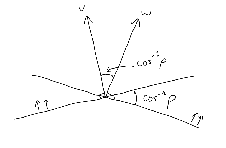
Without loss of generality $u$ is a unit vector. Then $⟨ x, u ⟩$ and $⟨ y, u ⟩$ are $ρ$ -correlated $1$ -dimensional Gaussians (by rotational invariance, we can think of $u$ as just being $u = e_{1}$ ).

So pick unit vectors $u, v \in ℝ^{2}$ , with $⟨ v, w ⟩ = ρ$ , and consider $⟨ v, g ⟩$ , $⟨ w, g ⟩$ , $g \sim N {(0, 1)}^{2}$ . Then draw a picture:

From this we get

ℙ [⟨ v, g ⟩ \geq 0 and ⟨ w, g ⟩ \geq 0] = \frac{π - \cos^{- 1} ρ}{2 π} = \frac{1}{2} - \frac{\cos^{- 1} ρ}{2 π} . □

A

is balanced (i.e. has Gaussian measure

\frac{1}{2}

), then

ℙ [x \in A, y \in A] = ℙ [x \notin A, y \notin A]

, so

The statement

{Stab}_{\cos δ} 𝟙_{A} (x) \leq \frac{1}{2} - \frac{δ}{2 π}

is equivalent to

{RS}_{δ} (A) \geq \frac{δ}{π}

Proof. For $i = 0, \dots, k$ , let $𝜃_{i} = δ_{1} + \dots + δ_{i}$ . Let $g$ and $g^{'}$ be independent $n$ -dimensional Gaussians and let $x_{i} = \cos 𝜃_{i} g + \sin 𝜃_{i} g^{'}$ for each $i$ . Then $x_{0}$ and $x_{k}$ are $\cos 𝜃_{k}$ -correlated, so

{RS}_{δ_{1} + \dots + δ_{k}} (A) = ℙ [𝟙_{A} (x_{0}) \neq 𝟙_{A} (x_{k})] .

Also, $x_{i - 1}$ and $x_{i}$ are ( $\cos 𝜃_{i - 1} \cos 𝜃_{i} + \sin 𝜃_{i - 1} \sin 𝜃_{i} = \cos (𝜃_{i} - 𝜃_{i - 1}) = \cos δ_{i}$ )-correlated. So the RHS equals $\sum_{i = 1}^{k} ℙ [𝟙_{A} (x_{i - 1}) \neq 𝟙_{A} (x_{i})]$ . The result now follows from a union bound. □

8 Invariance principles

Gaussian Space