4 Introduction to Fourier Restriction

Theorem (Hausdorff-Young inequality). Assuming that:

  • 1≤p≤2

  • 1p+1q=1

Then
∥f^∥q≤∥f∥p.

Proof. The inequality is true for p=1, q=∞ and for p=2, q=2 the inequality is true since we have equality (Plancherel).

For values in between we can interpolate. □

Are there any other (p,q) for which

∥f^∥q≲∥f∥p?(∗)

We saw that 1≤p≤2 was necessary (translations / modulations, Khinchin’s inequality).

Scaling: Plug in fλ(x)=f(λx) which is L∞-normalised (∥fλ∥∞=∥f∥∞). Then fλ^(ξ)=λ−nf^(λ−1ξ) which is L1-normalised (∥fλ^∥1=∥f^∥1).

(LHS of (∗))q=∫ℝn|fλ^(ξ)|qdξ=λ−nq+n∫|f^(ξ)|qdξ.
(RHS of (∗))p=∫ℝn|fλ(x)|pdx=λ−n∫|f(x)|pdx.

So we need for all λ>0:

λ−n+nq∥f^∥q≲λ−np∥f∥p.

So we need −n+nq=−np, i.e. 1p+1q=1.

Classical questions

What is Cp,q the smallest constant such that ∥f^∥q≤Cp,q∥f∥p?

Which functions f satisfy ∥f^∥q∥f∥p=Cp,q?

2014:

∥f^∥q≤Cp,q∥f∥p−dist⁡p(f,maximisers (Gaussian)).

Fourier restriction asks which (p,q) permit estimates ∥f^∥Lq(R)≲∥f∥Lp(ℝn) (R is the restricted frequency set, R⊆ℝn).

Example. R=B1(0)⊆ℝn, unit ball →: Basically, sitll governed by Hausdorff-Young inequality.

Example. R=B1(0)∩{xn=0} (measure 0 subset of ℝn).

RR(p→q) means

∥f^∥Lq(R)≲∥f∥Lp(ℝn)∀⁡f:ℝn→ℂ Schwartz

Always: RR(1→∞) true for all R.

In the second example, only this trivial statement is true (i.e. RR(p→q) is false for all other values for p,q).

Let R=Sn−1 be the unit sphere in ℝn. Consider

∥f^∥Lq(Sn−1)≲∥f∥Lp(ℝn)

where Lq(Sn−1) uses the usual surface measure dσ on Sn−1.

Notation.

^^ˇx↦→ −xf(x )       ^f(x)       f(x)        f(x)
     ◟◝◜◞        ◟◝◜◞       ◟◝◜◞        ◟◝◜◞
    ∈𝒮(ℝn)      ∈𝒮(ℝn)      ∈𝒮(ℝn)      ∈𝒮(ℝn)

We may call ˇ the “inverse Fourier transform”.

Let φ∈Cc∞(ℝn), ℝ-valued, ≥12 on B1(0), with support in B2(0).

May also assume ˇφ is ℝ-valued, ˇφ≳1 on Bc(0). ˇφ bounded, |ˇφ(x)|≲m(|x|2+1)−m∀⁡m. |ˇφ(x)| behaves like χB1(0) in Lp.

PIC

Consider dilates fR(x)=ˇφ(R−1x)e2πix⋅vr, R≫1.

Frequency side |fR^(ξ)|∼RnχBR−1(0)(x) (L1-norm).

PIC

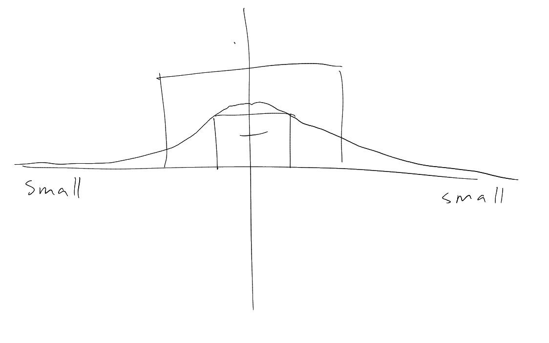
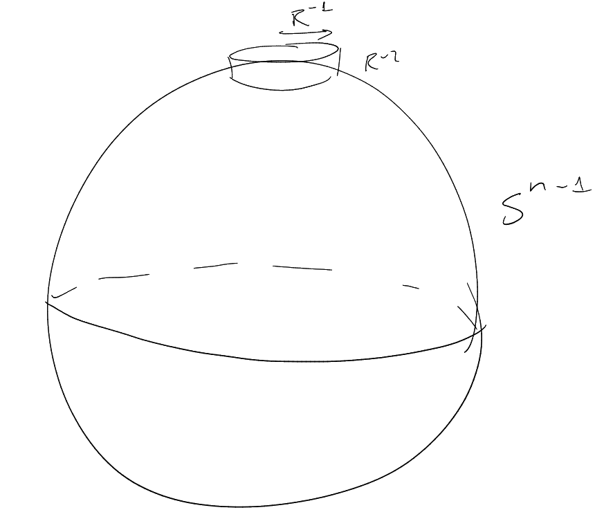
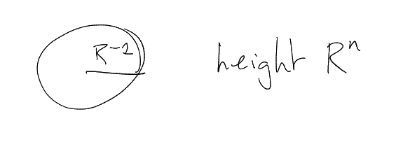
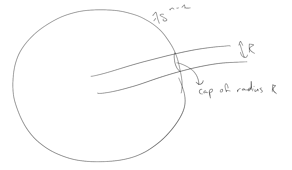
∫Sn−1|fR^(ξ)|qdσ(ξ)∼RnqR−(n−1)⏟→σ(BR−1(n)∩Sn−1).

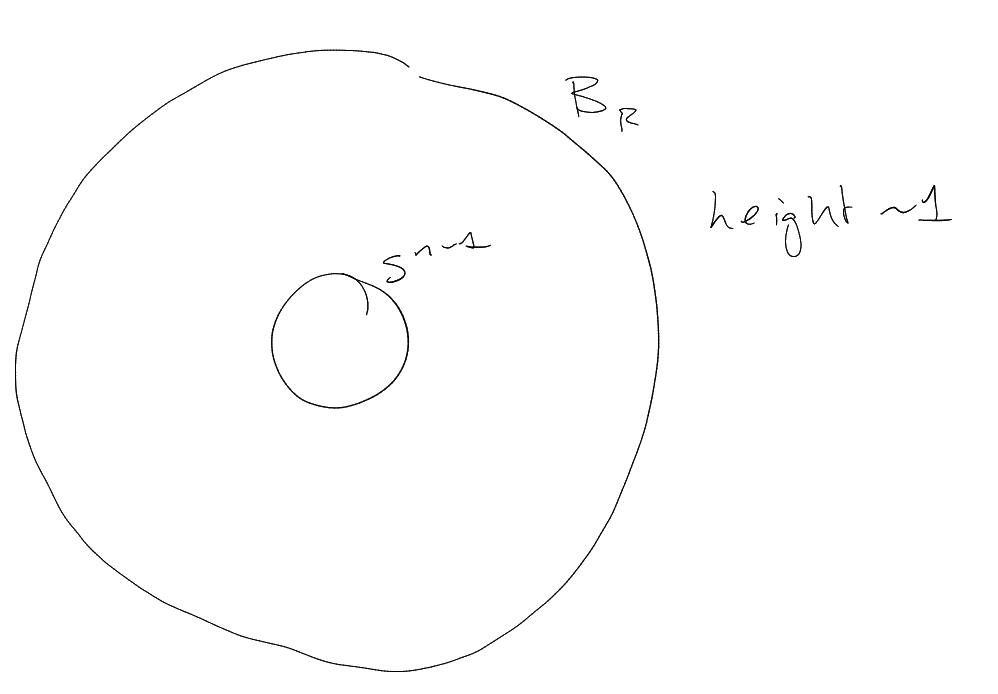
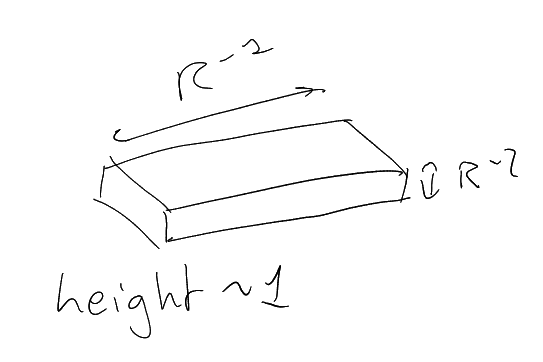
BR−1(n)∩Sn−1 cap of radius R−1. Spacial side |fR(x)|∼χBR(0)(x) (in L∞-norm).

PIC

height 1, ∫ℝn|fR(x)|pdx∼Rn.

Rn−n−1q≲Rnp, n−n−1q≤np.

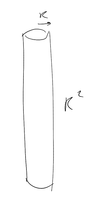
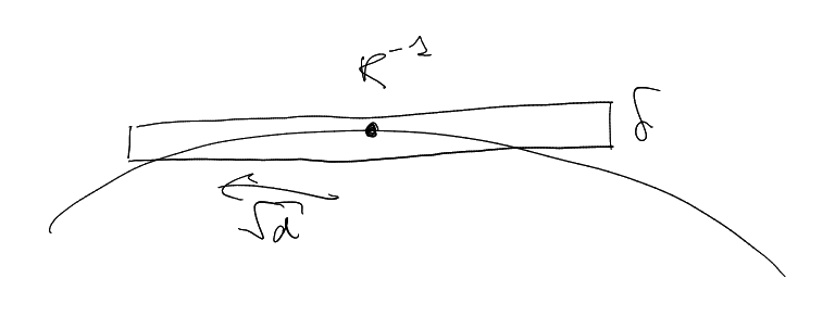
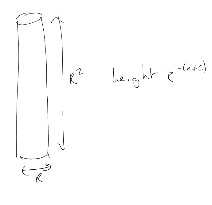
Consider: gR(x)=eix⋅wrˇφ(R−1x1,…,R−1xn−1,R−2xn).

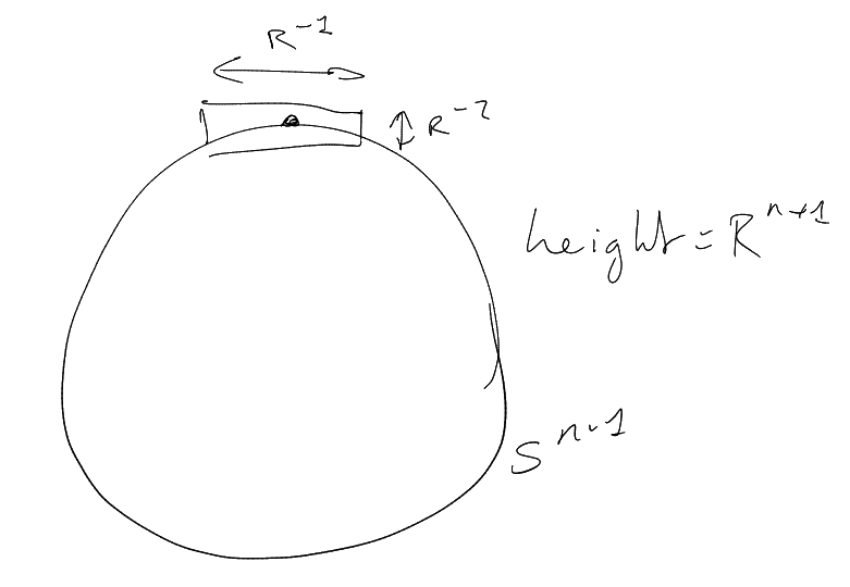
Frequency: |gr^(ξ)|≈|cylinder|−1χcylinder(ξ). |cylinder|−1| → (R−1⋅R−1R−2)−1=Rn+1.

PIC

∫Sn−1|gR^(ξ)|qdσ(ξ)∼R(n+1)qσ(cap of radius R−1)=R(n+1)q−(n−1).

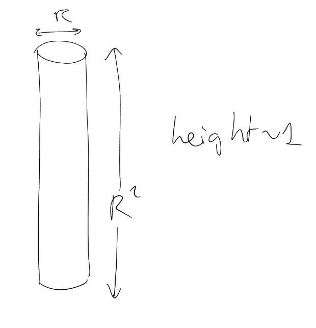
Spatial side: |gR′(x)|≈χcylinder(x) (L∞-norm).

PIC

∫|gR(x)|p=Rn−1+2=Rn+1.

→ Rn+1−n−1q≲Rn+1q, ⟹n+1−n−1q≤n+1p. Implies B.

On Monday, we will build examples h such that h^ sees all of Sn−1.

R=Sn−1⊆Rn.

Consider the statement

∥f^∥Lq(Sn−1)≲∥f∥Lp(ℝn).

(recall that we called this RSn−1(p→q)).

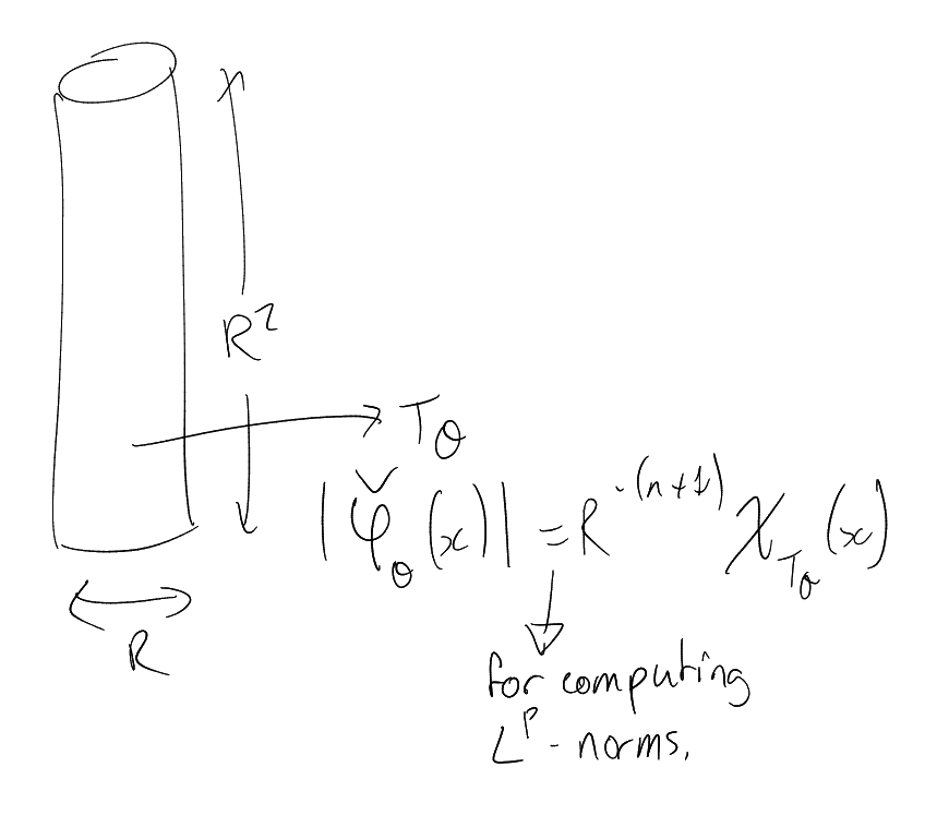
Fix φ∈Cc∞(ℝn), φ∼χB1(0). For computing Lp norms, |φ^|∼χBc(0).

Wave packet function with localised spatial and frequency behaviour.

Last time: fR(x)=eix⋅vRˇφ(R−1x1,…,R−1xn−1,R−2xn).

Frequency: |fR^(ξ)|

PIC

∫Sn−1|fR^|qdσ

n+1−n−1q≤n+1q

Spatial: |fR(x)|

PIC

∫ℝ1|fR|p

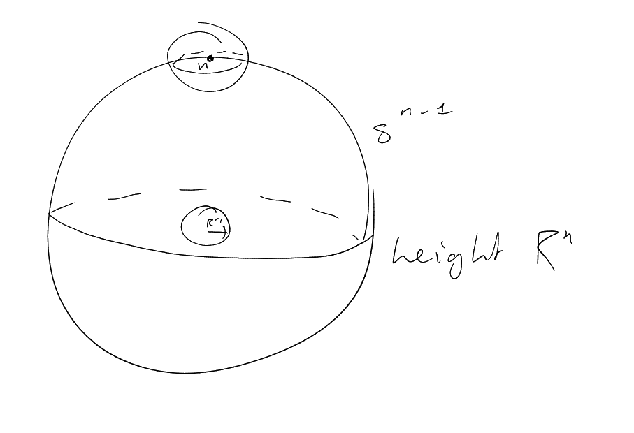
Note: sphere near n looks like (ξ1,1−12|ξ′|2), Sn−1∩supp⁡fR^∼cap of radius R−1.

PIC

Naive attempt: gR(x)=Rnˇφ(Rx)

Frequency: |gR^(ξ)|

PIC

∫Sn−1|gR^(ξ)|qdξ∼1

Spatial: |gR(x)|

PIC

∫|gR|p∼R−n⋅Rnp.

Deduce: 1≲R−np+n, so

p≥1

(trivial).

|gR^|∼1 on Sn−1 made ∥gR^∥Lq(Sn−1) easy to compute.

Could we improve things?

Could think about R∼1: then ∥gR^∥Lq(Sn−1)∼1, ∥gR∥p∼1. This is more efficient, but we can’t take a limit. So not so useful.

Build a function H(x) which satisfies |H^(ξ)|∼1 on Sn−1.

Let {𝜃} be a maximal collection of ∼R−1-spaced points on Sn−1 (#{𝜃}∼Rn−1).

PIC

For each 𝜃, let A𝜃−1:ℝn→ℝn be an affine map which sends

B1(0)→R−1×⋯×R−1×R−2 ellipsoid centered at 𝜃, tangent to Sn−1 at 𝜃.

Define φ𝜃=φ∘A𝜃, H(x)=∑⁡𝜃ˇφ𝜃(x).

H^(ξ)=∑⁡𝜃φ𝜃(ξ)∼1 on Sn−1 (actually on R−2-neighbourhood of Sn−1).

∫Sn−1|H^(ξ)|qdσ∼1.

H(x)=∑⁡𝜃ˇφ𝜃(x).

|φ𝜃(x)| Frequency:

PIC

|ˇφ𝜃(x)| Spatial:

PIC

ess⁡supp⁡H⊇⋃⁡𝜃ess⁡supp⁡ˇφ𝜃.

PIC

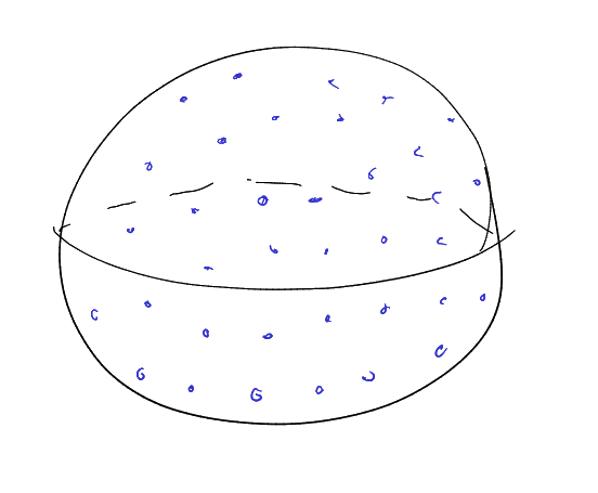
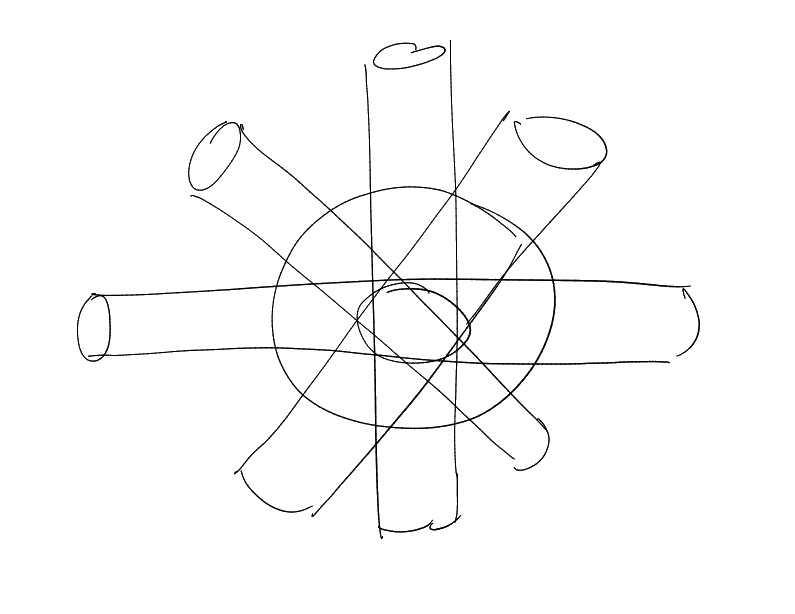
“bush of tubes”

∼Rn−1 many R×⋯×R×R2 tubes in R−1-separated directions

∫ℝn|H(x)|pdx=∫ℝn|∑𝜃ˇφ𝜃(x)⏟ℂ-valued function|pdx

PIC

Compute

∫ℝn|∑𝜃χT𝜃(x)2|p2=∫ℝn|∑𝜃χT𝜃(x)|p2=∫BR|∑χT𝜃|p2⏟(Rn−1)p2⋅Rn+∫RR2∖BR|∑χT𝜃|p2⏟(∗)

Consider overlap of T𝜃 on λSn−1 (λ∈(R,R2)).

Average overlap on λSn−1:

−∫λSn−1∑𝜃χT𝜃∼λ−(n−1)∑𝜃∫λSn−1χT𝜃∼λ−(n−1)∑𝜃Rn−1=λ−(n−1)R2(n−1).

PIC

Not too hard to check that the number of active T𝜃 on λSn−1 is ∼λ−(n−1)R2(n−1).

Now calculate:

(∗)∼∑R<λ<R2∫λ<|x|<2λ|∑𝜃χT𝜃|p2⏟[λ−(n−1)R2(n−1)]p2λndx.
1≲R−(n+1)p[R2n+R(n−1)p2Rn].

Two cases: either R2n dominates or the other term dominates. So p≤2nn+1.