Vector Calculus
February 4, 2022
Contents
1
Curves
1
1.1
Differentiating
the Curve . . . . .
1
Introduction
We will learn to differentiate and
integrate functions (or maps) of
the form
f :
m
n
R
→
R
|{z}
|{z}
domain
codomain
An element of
m
n
R
or R is a vec-
tor so this subject is called vector
calculus.
Examples of Maps
1. A function f :
n
R → R
defines a curve in
n
R . In
physics, we might think of
n
R as time and R
as phys-
ical space and write this as
f : t 7→ x(t)
with x ∈
n
R . (Obviously
we should take n = 3).
Generalising, a map
f :
2
n
R → R
defines a surface in
n
R , and
so on.
2. In
other
applications,
the domain
m
R
might be
viewed as physical space.
For example, in physics a
scalar field is a map
f :
3
R → R
for example temperature
T (x) is a scalar field, as is
the Higgs field.
A vector field is a map
f :
3
3
R
→
R
|{z}
|{z}
physical space
somethinge more abstract
for example the electric
field E(x) and magnetic
field B(x) are vector fields.
1
Curves
We consider maps of the form
f :
n
R → R
Assign a coordinate t to R and
use Cartesian coordinates on
n
R .
x = (x1, . . . , xn) = xiei
where ei is an orthonormal basis
such that ei · ej = δij. Note that
summation convention is used
here. (For
3
R
we also use nota-
tion {ei} = {ˆ
x, ˆ
y, ˆ
z}.)
The image of of the function f is
a parametrised curve x(t), with t
the parameter.
Examples
1. Consider the map
3
R → R
given by
x(t) = (at, bt2, 0)
The
curve
C
is
the
parabola a2y = bx2 in the
plane z = 0.
y
x
z
Note. When plotting
the curve, we lose in-
formation about the
parameter t.
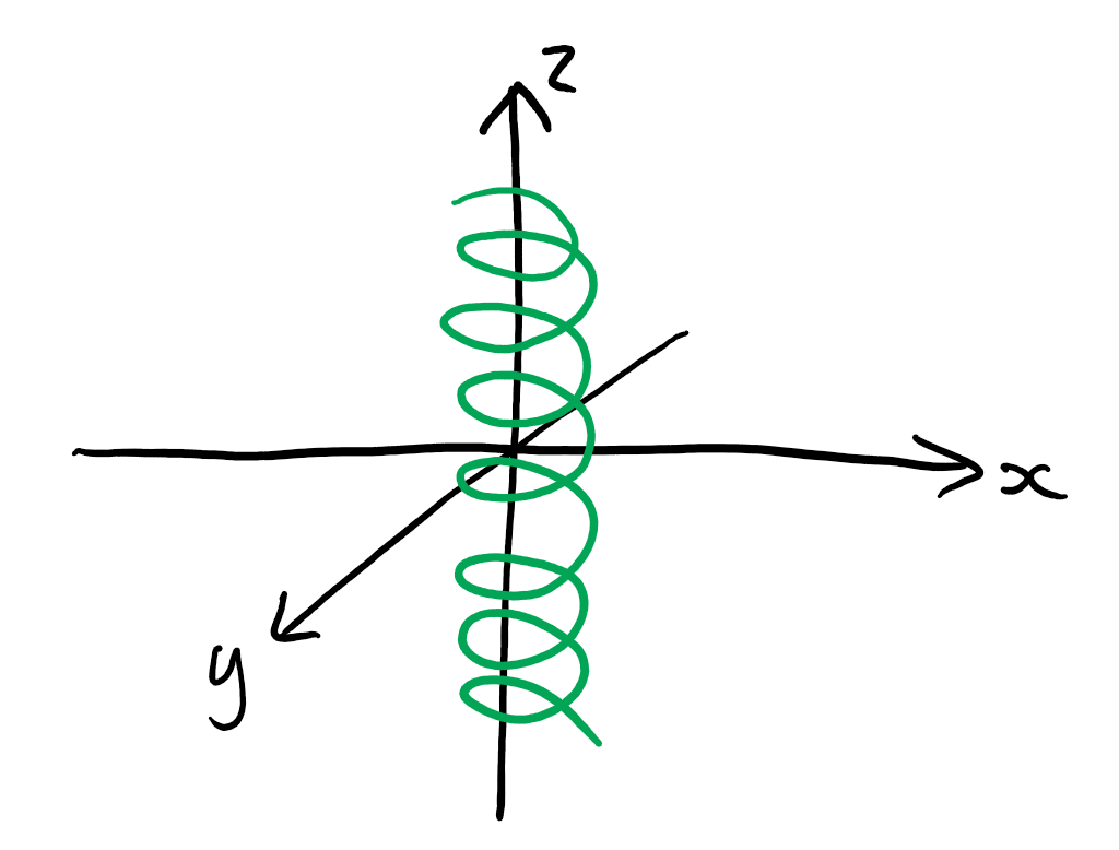
2. Consider
x(t)
=
(cos t, sin t, t)
The curve C is a helix.
The choice of parametrisation is
not unique, for example consider
x(t) = (cos λt, sin λt, λt).
This gives the same helix for all
λ ∈ R \ {0}.
Sometimes
the
choice
of
parametrisation
matters,
for
example if t is time and x(t)
is position, then the velocity
is proportional to λ.
But we
will see that some questions are
independent of the choice of
parametrisation.
1.1
Differentiating the
Curve
A vector function x(t) is differen-
tiable of t if, as δt → 0, we have
x(t+δt)−x(t) =
˙
x(t)δ(t)+O(δt2).
If
˙x(t)
exists
everywhere,
the
curve
is
said
to
be
smooth.
Note. “Big O” notation
O(δt2) means terms propor-
tional to δt2 or smaller.
In physics, dot is usually used
for time derivatives, for example
˙x(t) and prime for spatial deriva-
tives, for example f ′(x).
In maths, these are used inter-
changeably.
Some notation: we write
δx(t) = x(t + δt) − x(t)
The derivative is then
dx
δx
x ≡
:= lim
.
dt
δt→0 δt
Document Outline