
Logic and
Computability
Daniel Naylor
There are no non-experienced truths – L.E.J. Brouwer
Idea: a proof of is a “procedure” that comments a proof of into a proof of .
In particular, is not always the same as .
Fact: The law of excluded middle () is not generally intuitionistically valid.
Moreover, the Axiom of Choice is incompatible with intuitionistic set theory.
We take choice to mean that any family of inhabited sets admits a choice function.
Proof. Let be a proposition. By the Axiom of Separation, the following are sets (i.e. we can construct a proof that they are sets):
As and , we have that is a family of inhabited sets, thus admits a choice function by the Axiom of Choice. This satisfies and by definition.
Thus we have
and . Now means that and similarly for .
We can have the following:
So we can always specify a proof of or a proof of or a proof of . □
Why bother?
Intuitionistic maths is more general: we assume less.
Several notions that are conflated in classical maths are genuinely different constructively.
Intuitionistic proofs have a computable content that may be absent in classical proofs.
Intuitionistic logic is the internal logic of an arbitrary topos.
Let’s try to formalise the BHK interpretation of logic.
We will inductively define a provability relation by enforcing rules that implement the BHK interpretation.
We will use the notation to mean that is a consequence of the formulae in the set .
We obtain classical propositional logic (CPC) by adding either:
(reductio ad absurdum)
By
we mean ‘if we can prove assuming and we can prove assuming , then we can infer by “discharging / closing” the open assumptions and ’.
In particular, the (-I)-rule can be written as
We obtain intiuitionistic first-order logic (IQC) by adding rules for quantification:
If is a set of propositions in the language and is a proposition, we write , , , , if there is a proof of from in the respective logic.
Proof. Induction over the size of proofs. □
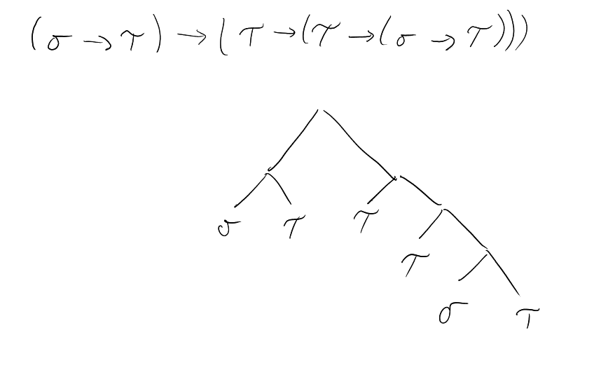
For now we assume given a set of simple types generated by a grammar
where is a countable set of type variables, as well as an infinite set of variables.
Definition 1.2.1 (Simply typed lambda-term). The set of simply typed -terms is defined by the grammar
A context is a set of pairs where the are (distinct) variables and each . We write for the set of all possible contexts. Given a context , we also write for the context (if does not appear in ).
The domain of is the set of variables that occur in it, and the range is the set of types that it manifests.
Definition 1.2.2 (Typability relation). We define the typability relation via:
Notation. We will refer to the -calculus of with this typability relation as .
A variable occurring in a -abstraction is bound, and it is free otherwise. We say that terms and are -equivalent if they differ only in the names of the bound variables.
If and are -terms and is a variable, then we define the substitution of for in by:
;
if ;
for -terms ;
, where and is not free in .
Definition 1.2.3 (beta-reduction). The -reduction relation is the smallest relation on closed under the following rules:
We also define -equivalence as the smallest equivalence relation containing .
When we reduce , the term being reduced is called a -redex, and the result is its -contraction.
Proof. Exercise. □
Lemma 1.2.7 (Substitution Lemma).
Notation. We will write if reduces to after (potentially multiple) -reductions.
Theorem 1.2.9 (Church-Rosser for lambda(->)). Assuming that:
Pictorially:
Corollary 1.2.10 (Uniqueness of normal form). If a simply typed -term admits a -normal form, then it is unique.
Proof.
Example 1.2.12. There is no way to assign a type to . If is of type , then in order to apply to , it has to be of type for some . But .
Definition 1.2.13 (Height). The height function is the recursively defined map that maps a type variable to , and a function type to .
We extend the height function from types to -redexes by taking the height of its -abstraction.
Not.: .
Proof (“Taming the Hydra”). The idea is to apply induction on the complexity of . Define a function by
where is the greatest height of a redex in , and is the number of redexes in of that height.
We will use induction over to show that if is typable, then it admits a reduction to -normal form.
Problem: reductions can copy redexes or create new ones.
Strategy: always reduce the right most redex of maximum height.
We will argue that by following this strategy, any new redexes we generate have to be lower than the height of the redex we picked to reduce.
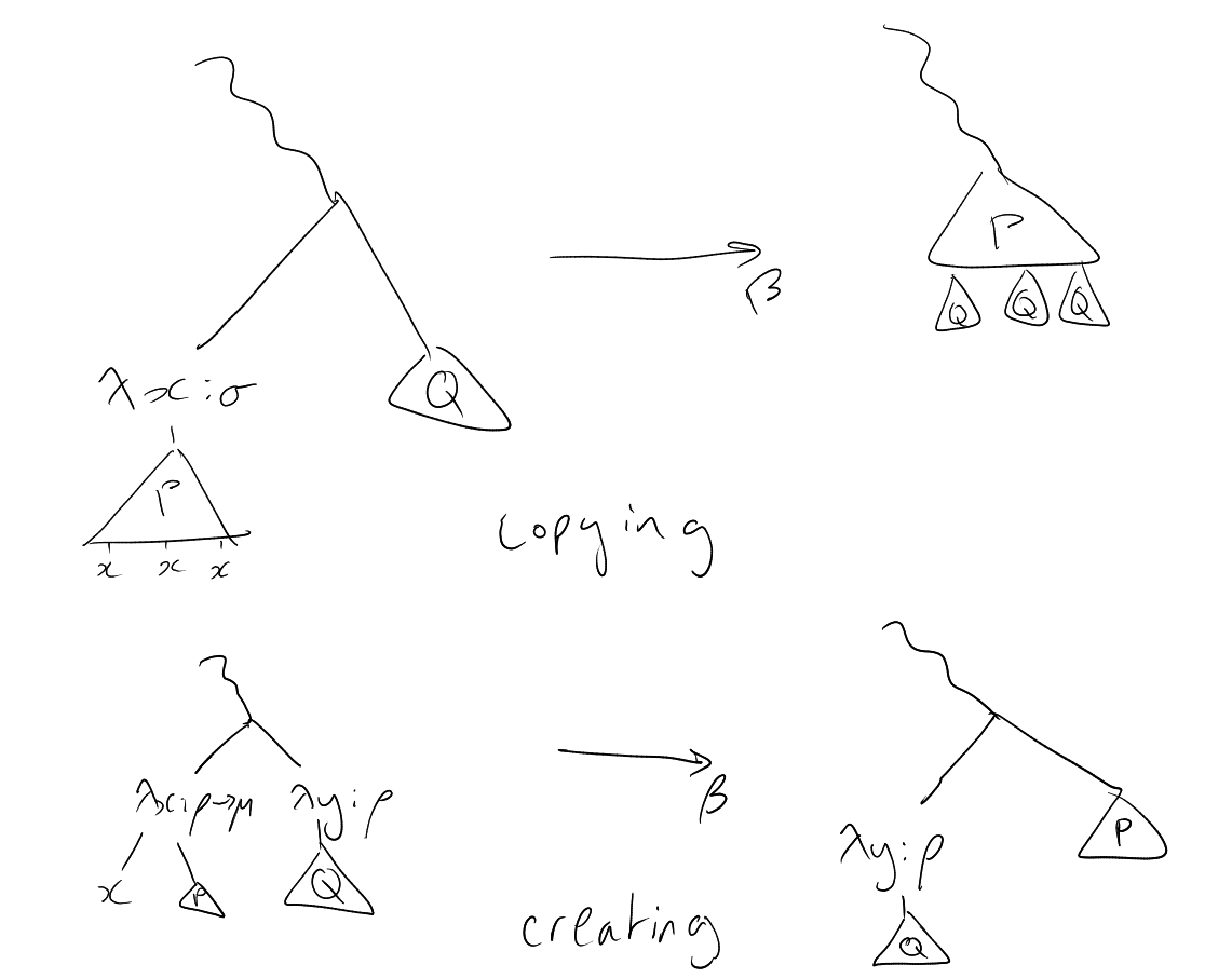
If and is already in -normal form, then claim is trivially true. If is not in -normal form, let be the rightmost redex of maximal height .
By reducing , we may introduce copies of existing redexes, or create new ones. Creation of new redexes of has to happen in one of the following ways:
Now itself is gone (lowering the count by ), and we just showed that any newly created redexes have height .
If we have and contains multiple free occurrences of , then all the redexes in are multiplied when performing -reduction.
However, our choice of ensures that the height of any such redex in has height , as they occur to the right of in . It is this always the case that (in the lexicographic order), so by the induction hypothesis, can be reduced to -normal form (and thus so can ). □
Proof. See Example Sheet 1. □
Propositions-as-types: idea is to think of as the “type of its proofs”.
The properties of the STC match the rules of IPC rather precisely.
First we will show a correspondence between and the implication fragment IPC of IPC that includes only the connective, the axiom scheme, and the and rules. We will later extend this to the whole of IPC by introducing more complex types to .
Start with IPC and build a STC out of it whose set of type variables is precisely the set of primitive propositions of the logic.
Clearly, the set of types then matches the set of propositions in the logic.
Proposition 1.3.1 (Curry-Howard for IPC(->)). Assuming that:
Proof.
If is a variable not occurring in and the derivation is of the form , then we’re supposed to prove that . But that follows from as .
If the derivation has of the form and , then we must have . By the induction hypothesis, we have that , i.e. . But then by (-I).
If the derivation has the form , then we must have and . By the induction hypothesis, we have that and , so by (-E).
Suppose the derivation is at a stage of the form
Then by the induction hypothesis, there are -terms and such that and , from which .
Finally, if the stage is given by
then we have two sub-cases:
If , then the induction hypothesis gives for some term . By weakening, we have , where does not occur in . But then as needed.
If , then the induction hypothesis gives for some , thus as needed. □
We have new typing rules:
for each
They come with new reduction rules:
Projections: and
Pairs:
Definition by cases: and
Unit: If , then
When setting up Curry-Howard with these new types, we let:
| STC | IPC |
| (primitive) types | (primitive) propositions |
| variable | hypothesis |
| ST-term | proof |
| type constructor | logical connective |
| term inhabitation | provability |
| term reduction | proof normalisation |
Definition 1.4.1 (Lattice). A lattice is a set equipped with binary commutative and associative operations and that satisfy the absorption laws:
for all .
A lattice is:
A Boolean algebra is a complemented distributive lattice.
Note that and are idempotent in any lattice. Moreover, we can define an ordering on by setting if .
Proof. Exercise. □
Classically, we say that if for every valuation with for all we have .
We might want to replace with some other Boolean algebra to get a semantics for IPC, with an accompanying Completeness Theorem. But Boolean algebras believe in the Law of Excluded Middle!
Definition 1.4.6 (Valuation in Heyting algebras). Let be a Heyting algebra and be a propositional language with a set of primitive propositions. An -valuation is a function , extended to the whole of recursively by setting:
A proposition is -valid if for all -valuations , and is an -consequence of a (finite) set of propositions if for all -valuations (written ).
Lemma 1.4.7 (Soundness of Heyting semantics). Assuming that:
Proof. By induction over the structure of the proof .
Example 1.4.8. The Law of Excluded Middle is not intuitionistically valid. Let be a primitive proposition and consider the Heyting algebra given by the topology on .
We can define a valuation with , in which case .
So . Thus Soundness of Heyting semantics implies that .
Classical completeness: if and only if .
Intuitionistic completeness: no single finite replacement for .
Definition (Lindenbaum-Tarski algebra). Let be a logical doctrine (CPC, IPC, etc), be a propositional language, and be an -theory. The Lindenbaum-Tarski algebra is built in the following way:
We’ll be interested in the case , , and .
Proposition 1.4.10. The Lindenbaum-Tarski algebra of any theory in is a distributive lattice.
Proof. Clearly, and inherit associativity and commutativity, so in order for to be a lattice we need only to check the absorption laws:
Equation () is true since by (-I), and also by (-E). Equation () is similar.
Now, for distributivity: by (-E) followed by (-E):
| (-E) | |
| (-E) | |
Conversely, by (-E) followed by (-I). □
Lemma 1.4.11. The Lindenbaum-Tarski algebra of any theory relative to IPC is a Heyting algebra.
Proof. We already saw that is a distributive lattice, so it remains to show that gives a Heyting implication, and that is bounded.
Suppose that , i.e. . We want to show that , i.e. . But that is clear:
| (hyp) | |
| (-I, ) | |
Conversely, if , then we can prove :
| (-E) | |
| (hyp) | |
| (-E) | |
So defining provides a Heyting .
The bottom element of is just : if is any element, then by -E.
The top element is : if is any proposition, then via
| (-E) | |
□
Theorem 1.4.12 (Completeness of the Heyting semantics). A proposition is provable in IPC if and only if it is -valid for every Heyting algebra .
Proof. One direction is easy: if , then there is a derivation in IPC, thus for any Heyting algebra and valuation , by Soundness of Heyting semantics. But then and is -valid.
For the other direction, consider the Lindenbaum-Tarski algebra of the empty theory relative to IPC, which is a Heyting algebra by Lemma 1.4.11. We can define a valuation by extending , to all propositions.
As is a valuation, it follows by induction (and the construction of ) that for all propositions.
Now is valid in every Heyting algebra, and so is valid in in particular. So , hence , hence . □
Given a poset , we can construct sets called principal up-sets.
Recall that is a terminal segment if for each .
Proposition 1.4.13. If is a poset, then the set can be made into a Heyting algebra.
Proof. Order the terminal segments by . Meets and joins are and , so we just need to define . If , define .
If , we have
which happens if for every and we have . But is a terminal segment, so this is the same as saying that . □
Definition 1.4.14 (Kripke model). Let be a set of primitive propositions. A Kripke model is a tuple where is a poset (whose elements are called “worlds” or “states”, and whose ordering is called the “accessibility relation”) and is a binary relation (“forcing”) satisfying the persistence property: if is such that and , then .
Every valuation on induces a Kripke model by setting is .
Definition 1.4.15 (Forcing relation). Let be a Kripke model for a propositional language. We define the extended forcing relation inductively as follows:
It is easy to check that the persistence property extends to arbitrary propositions.
Moreover:
if and only if for all .
if and only if for every , there exists with .
Notation. for a proposition if all worlds in force .
Example 1.4.16. Consider the following Kripke models:


In (1), we have , since and . We also know that , thus .
It is also the case that , yet , so either.
In (2), since can’t access a world that forces . Also either, as forces . So .
In (3), . All worlds force , and . So to check the claim we just need to verify that . But that is the case, as and .
Definition 1.4.17 (Filter). A filter on a lattice is a subset of with the following properties:
Exercise: a maximal proper filter (known as an ultra filter) is not principal if and only if it contains the Fréchet filter.
A filter is proper if .
A filter on a Heyting algebra is prime if it is proper and satisfies: whenever , we can conclude that or .
If is a proper filter and , then there is a prime filter extending that still doesn’t contain (by Zorn’s Lemma).
Proof (sketch). Let be the set of all prime filters of , ordered by inclusion. We write if and only if for primitive propositions .
We prove by induction that if and only if for arbitrary propositions.
For the implication case, say that and . Let be the least filter containing and . Then
Note that , or else for some , whence and so (as is a terminal segment).
In particular, is proper. So let be a prime filter extending that does not contain (exists by Zorn’s lemma).
By the induction hypothesis, , and since and (this ) contains , we have that . But then , contradiction.
This settles that implies .
Conversely, say that . By the induction hypothesis, , and so (as ). But then , as is a filter.
So the induction hypothesis gives , as needed.
The cases for the other connectives are easy ( needs primality). So is a Kripke model. Want to show that if and only if , for each .
Conversely, say , but . Since , there must be a proper filter that does not contain it. We can extend it to a prime filter that does not contain it, but then , contradiction. □
Proof. Soundness: induction over the complexity of .
Adequacy: Say . Then but for some Heyting algebra and -valuation (Theorem 1.4.12). But then Lemma 1.4.19 applied to and provides a Kripke model such that , but , contradicting the hypothesis on every Kripke model. □
Proof. Example Sheet 2. □
Lemma 1.5.3 (Regularisation). Assuming that:
Proof.
Define in . It is easy to show that this gives in (as preserves order), so is a Heyting algebra.
As every element of is regular (i.e. ), it is a Boolean algebra (see Example Sheet 2).
But we also have
Thus is a morphism of Boolean algebras. Note that any provides an element , since in . Additionally,
for all (as is in a Boolean algebra).
Now, if is a morphism of Boolean algebras with for all , then for all . So is unique with this property. □
In particular, if is a set, then .
Proof.
in , so .
Proof. Induction over the complexity of formulae. □
Corollary 1.5.6. CPC is inconsistent if and only if IPC is inconsistent.
Proof.
“If a ‘religion’ is defined to be a system of ideas that contains improvable statements, then Gödel taught us that mathematics is not only a religion; it is the only religion that can prove itself to be on.” – John Barrow
Definition 2.1.1 (Partial recursive function). The class of recursive functions is the smallest class of partial functions of the form that contains the basic functions:
and is closed under:
Notation: .
The class of functions produced by the same conditions but excluding minimisation is called the class of primitive recursive functions.
A partial recursive function that is defined everywhere is called a total recursive function.
The terms of the untyped -calculus are given by the grammar
where is a (countable) set of variables.
The notions we previously discussed (-equality, -reduction, -reduction, etc) apply tit for tat.
Example 2.1.2. Let and . Then . This shows that we can have an infinite reduction chain of -terms.
Question: If , , do we have and for some ?
Idea: “Simultaneously reduce” all the redexes in to get a term . This might have new redexes, so we can iterate the process to get terms .
should reduce to , so we have . We’ll see that if reduces to in steps, then .
Using this, we will show (assuming ):

To get there, we want to build with two properties:
Definition 2.1.3 (Takahashi Translation). The Takahashi translation of a -term is recursively defined as follows:
These rules are numbered by order of precedence, in case of ambiguity. We also define and .
Note that is not necessarily in -normal form, for example if , then
Proof. Induction over the structure of -terms. □
Lemma 2.1.5. Takahashi translation preserves -contraction:
Proof. By definition, . By induction over the structure of , we can check that:
If is not a -abstraction, then ,
If , then . □
Proof. Induction over the structure of . We’ll leave the easier cases as exercises, and focus on when is a redex, or when , where is not a -abstraction and with .
Suppose that is a redex. Then there are three possibilities for .
Now suppose , where is not a -abstraction, and with . Here . If is not a -abstraction, the result is clear. So let . Applying the induction hypothesis to , we get . Thus
Proof. Induction over the length of the chain , using Lemma 2.1.6. □
Applying this multiple times, implies for all .
Proof. By induction over . The base case is clear, as implies .
For , there is a term with . By induction hypothesis, . Since , we have by Lemma 2.1.4. Thus we get by the previous observation. Putting it all together:
Proof. Say , . Without loss of generality, say . By Theorem 2.1.8, we have that and . But by successive applications of Lemma 2.1.4 (as ). So take . □
Reminder of the picture to think of:

This has some important consequences:
If , then they to the same term;
If the -normal form of a term exists, it is unique;
We can use this to show that two terms are not -equivalent.
Example. and are different terms in -normal form, so they can’t be -equivalent.
Definition 2.1.10 (Church numeral). Let be a natural number. Its corresponding Church numeral is the -term , where denotes
Definition 2.1.12 (lambda-definability). A partial function is -definable if there is a -term such that .
Proof. We’ll show that , and leave the rest to you.
First note that
So:
In a similar fashion, we can also encode binary truth-values:
Proof. Just compute it! □
With this, we can encode logical connectives via:
;
;
.
We can also encode pairs: if we define , then and . However, it is not true that !
Recursively defining terms within the -calculus requires a clever idea: we see such a term as a solution to a fixed point equation where occurs somewhere in .
Theorem 2.1.15 (Fixed Point Theorem). There is a -term such that, for all :
Proof. Define
If we compute , we get:
We call any combinator (i.e. a -term without free variables) satisfying the property for all terms a fixed-point combinator.
Proof. Take . Then
Example 2.1.17. Suppose is a -term encoding a predicate, i.e. or for every . Let’s write down a -termthat encodes a program that takes a number and computes the next number satisfying the predicate.
First consider
where encodes the successor map. Our goal is to have run on itself. This can be done by using the term . Indeed:
for every .
Notation. will be short hand for (and the obvious generalisation to any number of variables, labelled in any way).
Lemma 2.1.18. The basic partial recursive functions are -definable.
Proof. The -th projection is definable by .
Successor is implemented by .
The zero map is given by .
Just compute! □
Lemma 2.1.19. The class of -definable functions is closed under composition.
Proof. Say is a -term defining , and that -terms define . Then the composite map is definable by the term
by inspection. □
Lemma 2.1.20. The class of -definable functions is closed under primitive recursion.
Proof. Suppose is obtained from and by primitive recursion.
and the -terms and define and respectively.
We need a -term to keep track of a pair that records the current state of computation: the value of and the value of at that stage.
So define
which acts on a pair by updating the iteration data. Then ought to be definable by
Indeed,
by definition of , and since
we have
as needed. □
Lemma 2.1.21. The -definable functions are closed under minimisation.
Proof. Suppose -defines , and that is defined from by minimisation: .
We can -define by implementing an algorithm that searches for the least in the following way:
First define a term that can check if a Church numeral is , for example
You can check that
Now we want a term that, on input , checks if and returns if so, else runs itself on . If we can do this, running it on input will perform the search.
Let:
and set
Note that
which is
Thus
if and
otherwise, as is -defined by . Hence
if is defined on . So -defines . □
Lemma 2.1.22. Every partial recursive function is -definable.
Definition 2.1.23 (Godel numbering). Let be a first-order language. A Gödel numbering is an injection that is:
Notation. We will use to be the Gödel numbering of an element of , for some fixed choice of Gödel numbering.
One way: assign a unique number to each symbol in your finite alphabet . We can then define
Remark. We can also encode proofs: add a symbol to the alphabet and code a proof with lines as .
Proof (sketch). Assign Gödel numbers to -terms . We can then consider a partial recursive function in that on input checks if is the Gödel numbering of a -term , and returns the Gödel numbering of its -normal form if it exists (undefined otherwise).
We also have partial recursive functions that convert to and vice-versa. Finally, say is a partial function defined by a -term . We can compute by first converting Church numerals to their Gödel numbers, then append the result to in order to get , then apply .
If is defined on , then has a -normal form, and what we get is . Otherwise is not defined.
We finish by going back from to . □
Recall that a subset is recursive (or decidable) if its characteristic map is total recursive.
Definition 2.2.1 (Recursively enumerable). We say that is recursively enumerable if any of the following are true:
Note, if and are both recursively enumerable, then is recursive. Note that the set of partial recursive function is countable, so we can fix an enumeration .
Example 2.2.2. The subset is recursively enumerable, but not recursive.
Definition 2.2.3 (Recursive / decidable language). A language is recursive if there is an algorithm that decides whether a string of symbols is an -formula.
An -theory is recursive if membership in is decidable (for -sentences).
An -theory is decidable if there is an algorithm for deciding whether .
We will work with recursive from now on.
Theorem 2.2.4 (Craig). Assuming that:
Proof. By hypothesis, there is a total recursive such that the axioms of are exactly .
Idea: Replace with something equivalent, but with a shape that lets us retrieve . Let
for each and
Then has the same deductive closure as . As formulae have finite length, we can check in finite time whether some is or some . By appropriate use of brackets, we can make sure that such an is “unique” if we are working with some .
In the first case, we halt and say we have a member of . In the second case, we check if , saying we have a member of if so, and that we don’t otherwise.
We can do this because we can scan the list and check symbol by symbol whether matches , which takes finite time.
If the input is not of the right shape, we halt and decide that it is . □
Lemma 2.2.5. The set of (Gödel numberings for) total recursive functions is not recursively enumerable.
Proof. Suppose otherwise, so there is a total recursive function whose image is the set of Gödel numberings of total recursive functions.
So for any total recursive , there is such that . Define by . This is certainly total recursive, but can’t be the function coded by for any , contradiction. □
Definition 2.2.6 (Language of arithmetic). The language of arithmetic is the first-order language with signature . The base theory of arithmetic is the -theory whose axioms express that:
The (first-order) theory of Peano arithmetic PA is obtained from by adding the scheme of induction: for each -formula , the axiom
Definition 2.2.7 (Delta0-formula, Sigma1-formula). A -formula of PA is one whose quantifiers are bounded, i.e. or , where is not free in and is quantifier free.
We say is a -formula if there is a -formula such that
It is a -formula if there is a -formula such that
In Example Sheet 4, you will prove that the characteristic function of a -definable set is partial recursive. We will show that the -definable sets are precisely the recursively enumerable ones.
Recall that defining yields a total recursive bijection .
Applying this a bunch of times, we get total recursive bijections by .
This is not good, as we have a different function for each . We’d like a “pairing function” that lets us see a number as a code for a sequence of any length.
This can be done within any model of PA by using a single function (known as Gödel’s -function) which is definable in PA.
We want an arithmetic procedure that can associate a code to sequences of any length, and such that the entries of the sequence can be recovered from the code.
We will do this by a clever application of the Chinese Remainder Theorem.
Suppose given a sequence of natural numbers. We want numbers to serve as moduli, with , and all of which are pairwise coprime. If we can find such that these conditions hold, then there is a number such that .
Taking works.
We say that the pair codes the sequence.
Remark. The forumula is given in PA by a -formula. We will use the notation for ; thus the decoding property is that if codes .
Proof.
The function is primitive recursive. By minimisation, the function
Since for tuples , we have that . Thus
as for each there is at most one such that . Now , so whenever defined. So is partial recursive.
The graphs of zero, successor, and -th projection are the formulae , , and respectively, so are -definable.
If and all have -graphs, then the graph of the composite is given by:
This is equal to a -formula, as those are closed under . If is obtained by primitive recursion
where and have -graphs, then we can use Godel’s Lemma to show that the graph of is given by
We do this by coding the sequence by . This formula is equal to a -formula since:
is equal to
as we can take to be the maximum between suitable with , , with .
A similar argument gives closure under minimisation.
If is and the graph of is definable by a -formula, then the graph of is definable by
by using Godel’s Lemma to code .
Again, this is equal to a -formula if the graph of is given by with , then is equal in to
Corollary 2.2.11. A subset is recursively enumerable if and only if there is a -formula such that, given , we have if and only if .
Proof.
Any model of PA includes a copy of inside of it: consider the standard natural numbers
In fact, embeds in any model PA as an initial segment: essentially because
In Example Sheet 4, you will see that is a -elementary substructure of any model of PA: every -sentence true in is also true in the model.
Definition 2.2.12 (Representation of a total function). Let be total and be any -theory extending PA. We say that is represented in if there is an formula such that, for all :
Lemma 2.2.13. Every total recursive function is -represented in PA.
Proof. The graph of is given by a -formula by Theorem 2.2.10, say where . Without loss of generality, we may assume that is a single variable (for example, rewrite ).
Let be the -formula
Then the -formula represents in PA.
We show first, where . Note that is the unique element of such that , as is a function.
Take to be the first natural number such that . Then too, whence . But any -sentence true in is true in any model of PA(c.f. Example Sheet 4), so , i.e. .
To see that , let be the first number such that , where . Suppose , with . We will show that . Completeness settles the claim. Again, is a -sentence true in , thus true in .
Using the fact that is a linear ordering in , we have , so (as is an initial segment of ). Now , hence and thus . Thus as needed. □
Corollary 2.2.14. Every recursive set is -representable in PA.
Proof. The characteristic function of is total recursive, so is represented by some -formula in PA. But then represents in PA. □
Lemma 2.2.15 (Diagonalisation Lemma). Assuming that:
Moreover, if is a -formula, then we can take to be a -sentence.
Proof. Define a total recursive function this way: on input , check if is the Gödel numbering of some -formula . If so, return , else return .
As is total recursive, it is -represented in by some . Consider the formula
Let and . This makes the sentence whose Gödel numbering is . It is obvious that , so we know that
Now represents in , and by construction, hence
Combining () and (), we get as needed.
Finally, note that if , then both and are equal to a -formula. □
Theorem 2.2.16 (Crude Incompleteness). Assuming that:
Proof. Let be a -formula that represents in PA, so that
This exists since is recursive. By the Diagonalisation Lemma, there is a -sentence such that .
If , then , and thus . But then (as and proves it).
If , then , so , and thus . As and , we have .
Since is consistent, we can’t have either of or in . □
Corollary 2.2.17 (Godel-Rosser Theorem). Let be a consistent -theory extending and admitting a recursively enumerable axiomatisation. Then is -incomplete: there is a -sentence such that and .
Proof. By Craig’s Theorem, we may assume that is recursive. Suppose that is -complete, and consider the set of (Gödel numberings of) all the and sentences in that proves.
The set is recursive: we can effectively decide if a given sentence is or , then check if by systematically searching through all proofs using the axioms in , until we either find a proof of or a proof of . Since is -complete, there is always such a proof, and we’ll find it in finite time.
But then satisfies the hypotheses of Theorem 2.2.16, so there is a -sentence with and , contradicting -completeness of . □
Definition 2.2.18 (Recursive structure). A (countable) -structure is recursive if there are total recursive functions , , a binary recursive relation , and natural numbers such that as -structures.
We will show that the usual is the only recursive model of (up to ).
Strategy:
Note that there is a -formula that captures being the -th prime, and . So if thinks that is the -th prime, then any model of thinks so too. Write for the -th prime.
Proof. Say for all standard , but only them. Then and holds (if holds, then and hence are standard).
By (induction), we conclude that . But is non-standard, so there is non-standard with , contradiction. □
Fix some , and a property of the natural numbers.
There is a number such that , namely the product of all primes with and .
We perceive as a code for the numbers with the property below , which we can decode by prime factorisation.
We could use other formulas to code subsets. Th subsets of coded in are those for which there is a -formula and such that .
As it turns out, coding via -formulae gives nothing new:
Proof (sketch*). The following formula holds in for any :
This is by the reasoning we gave when introducing codes, which works due to the bound on and . This can be proved in *.
Thus
for any . So by Lemma 2.2.19 there is a non-standard such that
So for any , there must be such that
Now is non-standard, so for all . So for any there is with
for all . □
Definition 2.2.22 (Recursively inseparable). We say that subsets are recursively inseparable if they are disjoint and there is no recursive with and .
Proposition 2.2.23. There are recursively enumerable subsets that are recursively inseparable.
Proof. Fix an effective enumeration of the partial recursive functions. Define and , which are clearly disjoint and are clearly recursively enumerable.
Suppose there is a recursive with and , and write for its (total recursive) characteristic function. There must be such that , as is total recursive.
Since and is either or , we have either or .
If , then , so , contradicting ; so . But then , so , contradicting . Thus and are recursively inseparable. □
Proof. Say are recursively enumerable and recursively inseparable. By Corollary 2.2.11, there are -formulae and defining and respectively (so and are -formulae).
Fix . As the sets are disjoint, we have:
As this sentence is , it follows, for any non-standard and that:
By Overspill, there is some non-standard such that
Now define . Note that:
: let , so that for some (a is defined by ). Then , as is . Hence as any standard is below as it is non-standard. But then .
: if , then for some , so arguing as before we get . By (), we can deduce . So .
As and are recursively inseparable, can’t be recursive. This shows that must encode a non-recursive set, which implies that it must canonically encode a non-recursive set by Proposition 2.2.21. □
Theorem 2.2.25 (Tennenbaum). Assuming that:
Proof. As is countable, we may as well assume that , , .
By Lemma 2.2.24, there is some that canonically codes a non-recursive subset .
As proves that
we have that
for all . So if and only if there is such that
Suppose is recursive. Then we can can through (which is ) and look for some that realises the disjunction of:
As is recursive, we can decide whether the disjunction holds of a given . Moreover, the search for such always terminates:
Euclidean division is provable in : for any with , there are unique such that and .
Combining these, we get that division of by in leaves a unique quotient , and remainder , which is either or or or …or ( times); i.e. one of the disjunctions from before.
Now we see that is recursive: if our search provides such that
then , and if the search gives satisfying one of the other disjunctions, then .
This contradicts the choice of , so can’t be recursive. □
˙
