Non-classical Logic - Logic and Computability

1 Non-classical Logic

There are no non-experienced truths – L.E.J. Brouwer

1.1 Intuitionistic Logic

Idea: a proof of $φ \to ψ$ is a “procedure” that comments a proof of $φ$ into a proof of $ψ$ .

In particular, $\neg \neg φ$ is not always the same as $φ$ .

Fact: The law of excluded middle ( $φ \lor \neg φ$ ) is not generally intuitionistically valid.

Moreover, the Axiom of Choice is incompatible with intuitionistic set theory.

We take choice to mean that any family of inhabited sets admits a choice function.

Theorem 1.1.1 (Diaconescu). The law of excluded middle can be intuitionistically deduced from the Axiom of Choice.

Proof. Let $φ$ be a proposition. By the Axiom of Separation, the following are sets (i.e. we can construct a proof that they are sets):

A : = {x \in {0, 1} : φ \lor (x = 0)} B : = {x \in {0, 1} : φ \lor (x = 1)} .

As $0 \in A$ and $1 \in B$ , we have that ${A, B}$ is a family of inhabited sets, thus admits a choice function $f : {A, B} \to A \cup B$ by the Axiom of Choice. This satisfies $f (A) \in A$ and $f (B) \in B$ by definition.

Thus we have

(f (A) = 0 \lor φ) \land (f (B) = 1 \lor φ)

and $f (A), f (B) \in {0, 1}$ . Now $f (A) \in {0, 1}$ means that $(f (A) = 0) \lor (f (A) = 1)$ and similarly for $f (B)$ .

We can have the following:

(1) We have a proof of $f (A) = 1$ , so $φ \lor (1 = 0)$ has a proof, so we must have a proof of $φ$ .
(2) We have a proof of $f (B) = 0$ , which similarly gives a proof of $φ$ .
(3) We have $f (A) = 0$ and $f (B) = 1$ , in which case we can prove $\neg φ$ : given a proof of $ϕ$ , we can prove that $A = B$ (by Extensionality), in which case $0 = f (A) = f (B) = 1$ , a contradiction.

So we can always specify a proof of $φ$ or a proof of $φ$ or a proof of $\neg φ$ . □

Why bother?

Intuitionistic maths is more general: we assume less.
Several notions that are conflated in classical maths are genuinely different constructively.
Intuitionistic proofs have a computable content that may be absent in classical proofs.
Intuitionistic logic is the internal logic of an arbitrary topos.

Let’s try to formalise the BHK interpretation of logic.

We will inductively define a provability relation by enforcing rules that implement the BHK interpretation.

We will use the notation $Γ ⊢ φ$ to mean that $φ$ is a consequence of the formulae in the set $Γ$ .

Rules for Intuitionistic Propositional Calculus (IPC)

( $\land$ -I) $\frac{Γ ⊢ A, Γ ⊢ B}{Γ ⊢ A \land B}$
( $\lor$ -I) $\frac{Γ ⊢ A}{Γ ⊢ A \lor B}$ , $\frac{Γ ⊢ B}{Γ ⊢ A \lor B}$
( $\land$ -E) $\frac{Γ ⊢ A \land B}{Γ ⊢ A}$ and $\frac{Γ ⊢ A \land B}{Γ ⊢ B}$
( $\lor$ -E) $\frac{Γ, A ⊢ C Γ, B ⊢ C Γ ⊢ A \lor B}{Γ ⊢ C}$
( $\to$ -I) $\frac{Γ, A ⊢ B}{Γ ⊢ A \to B}$
( $\to$ -E) $\frac{Γ ⊢ A \to B, Γ ⊢ A}{Γ ⊢ B}$
( $⊥$ -E) $\frac{Γ ⊢ ⊥}{Γ ⊢ A}$ for any $A$
(Ax) $\frac{}{Γ, A ⊢ A}$ for any $A$
(Weak) $\frac{Γ ⊢ B}{Γ, A ⊢ B}$
(Contr) $\frac{Γ, A, A ⊢ B}{Γ, A ⊢ B}$

We obtain classical propositional logic (CPC) by adding either:

$\frac{}{Γ ⊢ A \lor \neg A}$
$\frac{Γ, \neg A ⊢ ⊥}{Γ ⊢ A}$ (reductio ad absurdum)

\frac{\begin{matrix} [A] \\ ⋮ \\ X \end{matrix} \begin{matrix} [B] \\ ⋮ \\ Y \end{matrix}}{C} (A, B)

we mean ‘if we can prove $X$ assuming $A$ and we can prove $Y$ assuming $B$ , then we can infer $C$ by “discharging / closing” the open assumptions $A$ and $B$ ’.

In particular, the ( $\to$ -I)-rule can be written as

\frac{\begin{matrix} Γ, [A] \\ ⋮ \\ B \end{matrix}}{Γ ⊢ A \to B} (A) .

We obtain intiuitionistic first-order logic (IQC) by adding rules for quantification:

( $\exists$ -I) $\frac{Γ ⊢ φ [x : = t]}{Γ ⊢ \exists x . φ (x)}$ , where $t$ is a term.
( $\exists$ -E) $\frac{Γ ⊢ \exists x . φ Γ, φ ⊢ ψ}{Γ ⊢ ψ}$ , if $x$ is not free in $Γ, ψ$ .
( $\forall$ -I) $\frac{Γ ⊢ φ}{Γ ⊢ \forall x . φ}$ if $x$ is not free in $Γ$ .
( $\forall$ -E) $\frac{Γ ⊢ \forall x . φ (x)}{Γ ⊢ φ [x : = t]}$ , where $t$ is a term.

Example 1.1.2. Let’s give a natural deduction proof of $A \land B \to B \land A$ .

\frac{\frac{\frac{[A \land B]}{A} \frac{[A \land B]}{B}}{B \land A}}{A \land B \to B \land A} (A \land B) .

Example 1.1.3. Let’s prove the Hilbert-style axioms $φ \to (ψ \to φ)$ and $(φ \to (ψ \to χ)) \to ((φ \to p s i) \to (φ \to χ))$ .

\frac{\frac{[φ] [ψ]}{ψ \to φ} (ψ)}{φ \to (ψ \to φ)} (φ)

$[φ \to (ψ \to χ)] [φ \to ψ] [φ]$	(toE)

$ψ \to χ ψ$	(toE)

$χ$	(toI,ψ)

$φ \to χ$	(toI, φ→ψ)

$(φ \to ψ) \to (φ \to χ)$	(toI, (φ→(ψ→χ)))

$(φ \to (ψ \to χ)) \to ((φ \to ψ) \to (φ \to χ))$

If $Γ$ is a set of propositions in the language and $φ$ is a proposition, we write $Γ ⊢_{IPC} φ$ , $Γ ⊢_{IQC} φ$ , $Γ ⊢_{CPC} φ$ , $Γ ⊢_{CQC} φ$ , if there is a proof of $φ$ from $Γ$ in the respective logic.

Lemma 1.1.4. Assuming that:

$Γ ⊢_{IPC} φ$
$ψ$ a proposition

Then

Γ, ψ ⊢_{IPC} φ

. Moreover, if

p

is a primitive proposition and

ψ

is any proposition, then

Γ [p : = ψ] ⊢_{IPC} φ [p : = ψ] .

Proof. Induction over the size of proofs. □

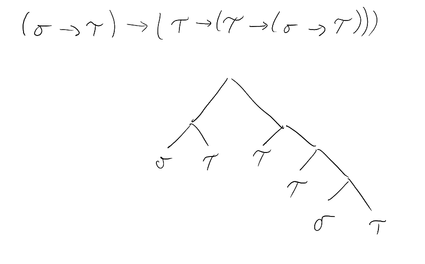
1.2 The simply typed $λ$ -calculus

For now we assume given a set $Π$ of simple types generated by a grammar

Π : = U | Π \to Π,

where $U$ is a countable set of type variables, as well as an infinite set $V$ of variables.

Definition 1.2.1 (Simply typed lambda-term). The set $Λ_{Π}$ of simply typed $λ$ -terms is defined by the grammar

Λ_{Π} : = \underset{variables}{\underset{⏟}{V}} | \underset{λ -abstraction}{\underset{⏟}{λ V : Π . Λ_{Π}}} | \underset{λ -application}{\underset{⏟}{Λ_{Π} Λ_{Π}}} .

A context is a set of pairs ${x_{1} : τ_{1}, \dots, x_{n} : τ_{n}}$ where the $x_{i}$ are (distinct) variables and each $τ_{i} \in Π$ . We write $C$ for the set of all possible contexts. Given a context $Γ \in C$ , we also write $Γ, x : τ$ for the context $Γ \cup {x : τ}$ (if $x$ does not appear in $Γ$ ).

The domain of $Γ$ is the set of variables that occur in it, and the range $| Γ |$ is the set of types that it manifests.

Definition 1.2.2 (Typability relation). We define the typability relation $⊩ \subseteq C \times Λ_{Π} \times Π$ via:

(1)
For every context $Γ$ , and variable $x$ not occurring in $Γ$ , and type $τ$ , we have $Γ, x : τ ⊩ x : τ$ .
(2)
Let $Γ$ be a context, $x$ a variable not occurring in $Γ$ , and let $σ, τ \in Π$ be types, and $M$ be a $λ$ -term. If $Γ, x : σ ⊩ M : τ$ , then $Γ ⊩ (λ x : σ . M) : (σ \to τ)$ .
(3)
Let $Γ$ be a context, $σ, τ \in Π$ be types, and $M, N \in Λ_{Π}$ be terms. If $Γ ⊩ M : (σ \to τ)$ and $Γ ⊩ N : σ$ , then $Γ ⊩ (M N) : τ$ .

Notation. We will refer to the $λ$ -calculus of $Λ_{Π}$ with this typability relation as $λ (\to)$ .

A variable $x$ occurring in a $λ$ -abstraction $λ \underset{̲}{x} : σ . M$ is bound, and it is free otherwise. We say that terms $M$ and $N$ are $α$ -equivalent if they differ only in the names of the bound variables.

If $M$ and $N$ are $λ$ -terms and $x$ is a variable, then we define the substitution of $N$ for $x$ in $M$ by:

$x [x : = N] = N$ ;
$y [x : = N] = y$ if $x \neq y$ ;
$(P Q) [x : = N] = P [x : = N] Q [x : = N]$ for $λ$ -terms $P, Q$ ;
$(λ y : σ . P) [x : = N] = λ y : σ . (P [x : = N])$ , where $x \neq y$ and $y$ is not free in $N$ .

Definition 1.2.3 (beta-reduction). The $β$ -reduction relation is the smallest relation $\to_{β}$ on $Λ_{Π}$ closed under the following rules:

$(λ x : σ . P) Q \to_{β} P [x : = Q]$ ,
if $P \to_{β} P^{'}$ , then for all variables $x$ and types $σ \in Π$ , we have $λ x : σ . P \to_{β} λ x : σ . P^{'}$ ,
$P \to_{β} P^{'}$ and $z$ as a $λ$ -term, then $P Z \to_{β} P^{'} Z$ and $Z P \to_{β} Z P^{'}$ .

We also define $β$ -equivalence $\equiv_{β}$ as the smallest equivalence relation containing $\to_{β}$ .

Example 1.2.4 (Informal). We have $(λ x : ℤ . (λ y : τ . x)) Z \to_{β} (λ y : τ . Z)$ .

When we reduce $(λ x : σ . P) Q$ , the term being reduced is called a $β$ -redex, and the result is its $β$ -contraction.

Lemma 1.2.5 (Free variables lemma). Assuming that:

$Γ ⊩ M : σ$

Then

(1) If $Γ \subseteq Γ^{'}$ , then $Γ^{'} ⊩ M : σ$ .
(2) The free variables of $M$ occur in $Γ$ .
(3) There is a context $Γ^{*} \subseteq Γ$ comprising exactly the free variables in $M$ , with $Γ^{*} ⊩ M : σ$ .

Proof. Exercise. □

Lemma 1.2.6 (Generation Lemma).

(1)
For every variable $x$ , context $Γ$ , and type $σ$ , if $Γ ⊩ x : σ$ , then $x : σ \in Γ$ ;
(2)
If $Γ ⊩ (M N) : σ$ , then there is a type $τ$ such that $Γ ⊩ M : τ \to σ$ and $Γ ⊩ N : τ$ ;
(3)
If $Γ ⊩ (λ x . M) : σ$ , then there are types $τ$ and $ρ$ such that $Γ, x : τ ⊩ M : ρ$ and $σ = (τ \to ρ)$ .

Lemma 1.2.7 (Substitution Lemma).

(1)
If $Γ ⊩ M : σ$ and $α$ is a type variable, then $Γ [α : = τ] ⊩ M : σ [α : = τ]$ ;
(2)
If $Γ, x : τ ⊩ M : σ$ and $Γ ⊩ N : τ$ , then $Γ ⊩ M [x : = N] : σ$ .

Proposition 1.2.8 (Subject reduction). Assuming that:

$Γ ⊩ M : σ$
$M \to_{β} N$

Then

Γ ⊩ N : σ

Proof. By induction on the derivation of $M \to_{β} N$ , using Lemma 1.2.6 and Lemma 1.2.7. □

Notation. We will write $M ↠_{β} N$ if $M$ reduces to $N$ after (potentially multiple) $β$ -reductions.

Theorem 1.2.9 (Church-Rosser for lambda(->)). Assuming that:

$Γ ⊩ M : σ$
$M ↠_{β} N_{1}$
$M ↠_{β} N_{2}$

Then there is a

λ

-term

L

such that

N_{1} ↠_{β} L

N_{2} ↠_{β} L

, and

Γ ⊩ L : σ

Pictorially:

Definition ( $b e t a$ -normal form). A $λ$ -term $M$ is in $β$ -normal form if there is no term $N$ such that $M \to_{β} N$ .

Corollary 1.2.10 (Uniqueness of normal form). If a simply typed $λ$ -term admits a $β$ -normal form, then it is unique.

Proposition 1.2.11 (Uniqueness of types).

(1)
If $Γ ⊩ M : σ$ and $Γ ⊩ M : τ$ , then $σ = τ$ .
(2)
If $Γ ⊩ M : σ$ , $Γ ⊩ N : τ$ , and $M \equiv_{β} N$ , then $σ = τ$ .

Proof.

(1) Induction.
(2) By the hypothesis and Church-Rosser for lambda(->), there is a term $L$ which both $M$ and $N$ reduce to. By Lemma 1.2.7, we have $Γ ⊩ L : σ$ and $Γ ⊩ L : τ$ , so $σ = τ$ by (1). □

Example 1.2.12. There is no way to assign a type to $λ x : x . x$ . If $x$ is of type $τ$ , then in order to apply $x$ to $x$ , it has to be of type $τ \to σ$ for some $σ$ . But $τ \neq τ \to σ$ .

Definition 1.2.13 (Height). The height function is the recursively defined map $h : Π \to ℕ$ that maps a type variable to $0$ , and a function type $σ \to τ$ to $1 + \max (h (σ), h (τ))$ .

We extend the height function from types to $β$ -redexes by taking the height of its $λ$ -abstraction.

Not.: ${(λ x : σ . P^{τ})}^{σ \to τ} R^{σ}$ .

Theorem 1.2.14 (Weak normalisation for lambda(->)). Assuming that:

$Γ ⊩ M : σ$

Then there is a finite reduction path

M : = M_{0} \to_{β} M_{1} \to_{β} M_{2} \to_{β} \dots \to_{β} M_{n}

, where

M_{n}

is in

β

-normal form.

Proof (“Taming the Hydra”). The idea is to apply induction on the complexity of $M$ . Define a function $m : Λ_{Π} \to ℕ \times ℕ$ by

m (M) = {\begin{matrix} (0, 0) & if M is in β -normal form \\ (h (M), r e d e x (M)) & otherwise \end{matrix},

where $h (M)$ is the greatest height of a redex in $M$ , and $r e d e x (M)$ is the number of redexes in $M$ of that height.

We will use induction over $ω \times ω$ to show that if $M$ is typable, then it admits a reduction to $β$ -normal form.

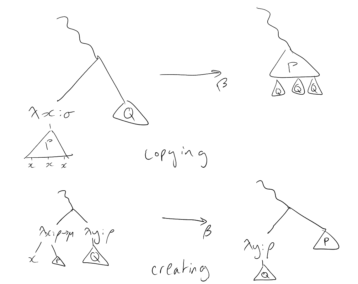
Problem: reductions can copy redexes or create new ones.

Strategy: always reduce the right most redex of maximum height.

We will argue that by following this strategy, any new redexes we generate have to be lower than the height of the redex we picked to reduce.

If $Γ ⊩ M : σ$ and $M$ is already in $β$ -normal form, then claim is trivially true. If $M$ is not in $β$ -normal form, let $Δ$ be the rightmost redex of maximal height $h$ .

By reducing $Δ$ , we may introduce copies of existing redexes, or create new ones. Creation of new redexes of $Δ$ has to happen in one of the following ways:

(1) If $Δ$ is of the form $(λ x : (ρ \to μ) \dots x P^{ρ} \dots) {(λ y : ρ . Q^{μ})}^{P \to μ}$ , then it reduces to $\dots {(λ y : ρ . Q^{μ})}^{ρ \to μ} P^{μ} \dots$ , in which case there is a new redex of height $h (ρ \to μ) < h$ .
(2) We have $Δ = (λ x : τ . (λ y : ρ . R^{μ})) P^{τ}$ occurring in $M$ in the scenario $Δ^{ρ \to μ} Q^{ρ}$ . Say $Δ$ reduces to $λ y : ρ . R_{1}^{μ}$ . Then we create a new redex of height $h (ρ \to μ) < h (τ \to (ρ \to μ)) = h$ .
(3) The last possibility is that $Δ = (λ x : (ρ \to μ) . x) (λ y : ρ . P^{μ})$ , and that it occurs in $M$ as $Δ^{ρ \to μ} Q^{ρ}$ . Reduction then gives the redex ${(λ y : ρ . P^{μ})}^{ρ \to μ} Q^{ρ}$ of height $h (ρ \to μ) < h$ .

Now $Δ$ itself is gone (lowering the count by $1$ ), and we just showed that any newly created redexes have height $< h$ .

If we have $Δ = (λ x : τ . P^{ρ}) Q^{τ}$ and $P$ contains multiple free occurrences of $x$ , then all the redexes in $Q$ are multiplied when performing $β$ -reduction.

However, our choice of $Δ$ ensures that the height of any such redex in $Q$ has height $< h$ , as they occur to the right of $Δ$ in $M$ . It is this always the case that $m (M^{'}) < m (M)$ (in the lexicographic order), so by the induction hypothesis, $M^{'}$ can be reduced to $β$ -normal form (and thus so can $M$ ). □

Theorem 1.2.15 (Strong Normalisation for lambda(->)). Assuming that:

$Γ ⊩ M : σ$

Then there is no infinite reduction sequence

M \to_{β} M_{1} \to_{β} \dots

Proof. See Example Sheet 1. □

1.3 The Curry-Howard Correspondence

Propositions-as-types: idea is to think of $φ$ as the “type of its proofs”.

The properties of the ST $λ$ C match the rules of IPC rather precisely.

First we will show a correspondence between $λ (\to)$ and the implication fragment IPC $(\to)$ of IPC that includes only the $\to$ connective, the axiom scheme, and the $(\to - I)$ and $(\to - E)$ rules. We will later extend this to the whole of IPC by introducing more complex types to $λ (\to)$ .

Start with IPC $(\to)$ and build a ST $λ$ C out of it whose set of type variables $U$ is precisely the set of primitive propositions of the logic.

Clearly, the set $Π$ of types then matches the set of propositions in the logic.

Comment: $λ x : σ . (M x) \to_{η} M$ if $x$ is not free in $M$ .

Proposition 1.3.1 (Curry-Howard for IPC(->)). Assuming that:

$Γ$ is a context for $λ (\to)$
$φ$ a proposition

Then

(1) If $Γ ⊩ M : φ$ , then $| Γ | = {τ \in Π : (x : τ) \in Γ for some x} ⊢_{IPC(\to)} φ$
(2) If $| Γ | ⊢_{IPC(\to)} φ$ , then there is a simply typed $λ$ -term $M \in λ (\to)$ such that ${(x_{ψ} : ψ) | ψ \in Γ} ⊩ M : φ$ .

Proof.

(1) We induct over the derivation of $Γ ⊩ M : φ$ .
If $x$ is a variable not occurring in $Γ^{'}$ and the derivation is of the form $Γ^{'}, x : φ ⊩ x : φ$ , then we’re supposed to prove that $| Γ^{'}, x : φ | ⊢ φ$ . But that follows from $φ ⊢ φ$ as $| Γ^{'}, x : φ | = | Γ^{'} | \cup {φ}$ .

If the derivation has $M$ of the form $λ x : σ . N$ and $φ = σ \to τ$ , then we must have $Γ, x : σ ⊩ N : τ$ . By the induction hypothesis, we have that $| Γ, x : σ | ⊢ τ$ , i.e. $| Γ |, σ ⊢ τ$ . But then $| Γ | ⊢ σ \to τ$ by ( $\to$ -I).

If the derivation has the form $Γ ⊩ (P Q) : φ$ , then we must have $Γ ⊩ P : (σ \to φ)$ and $Γ ⊩ Q : σ$ . By the induction hypothesis, we have that $| Γ | ⊢ σ \to φ$ and $| Γ | ⊢ σ$ , so $| Γ | ⊢ φ$ by ( $\to$ -E).
(2) Again, we induct over the derivation of $Γ ⊢ φ$ . Write $Δ = {(x_{ψ} : ψ) | ψ \in Γ}$ . Then we only have a few ways to construct a proof at a given stage. Say the derivation is of the form $Γ, φ ⊢ φ$ . If $φ \in Γ$ , then clearly $Δ ⊩ x_{φ} : φ$ , and if $φ \notin Γ$ then $Δ, x_{φ} : φ ⊩ x_{φ} : φ$ .
Suppose the derivation is at a stage of the form
$\frac{Γ ⊢ φ \to ψ Γ ⊢ φ}{Γ ⊢ ψ} .$

Then by the induction hypothesis, there are $λ$ -terms $M$ and $N$ such that $Δ ⊩ M : (φ \to ψ)$ and $Δ ⊩ N : φ$ , from which $Δ ⊩ (M N) : φ$ .

Finally, if the stage is given by
$\frac{Γ, φ ⊢ ψ}{Γ ⊢ φ \to ψ},$

then we have two sub-cases:
- If $φ \in Γ$ , then the induction hypothesis gives $Δ ⊩ M : ψ$ for some term $M$ . By weakening, we have $Δ, x : φ ⊩ M : ψ$ , where $x$ does not occur in $Δ$ . But then $Δ ⊩ (λ x : φ . M) : (φ \to ψ)$ as needed.
- If $φ \notin Γ$ , then the induction hypothesis gives $Δ, x_{φ} : φ ⊩ M : ψ$ for some $M$ , thus $Δ ⊩ (λ x_{φ} : φ . M) : (φ \to ψ)$ as needed. □

Example 1.3.2. Let $φ, ψ$ be primitive propositions. The $λ$ -term

λ f : (φ \to ψ) \to φ . λ : φ \to ψ . \overset{ψ}{\overset{︷}{g (\underset{φ}{\underset{⏟}{f g}})}}

has type $((φ \to ψ) \to φ) \to ((φ \to ψ) \to ψ)$ , and therefore encodes a proof of that proposition in IPC( $\to$ ).

$g : φ \to ψ$ , $f : (φ \to ψ) \to φ$ .

$g : [φ \to ψ] f : [(φ \to ψ) \to φ]$	(toE)

$f g : φ g : [φ \to ψ]$	(toE)

$g (f g) : ψ$	(toI, φ→ψ)

$λ g . g (f g) : (φ \to ψ) \to ψ$	(toI, (φ→ψ) →φ)

$λ f . λ g . g (f g) : ((φ \to ψ) \to φ) \to ((φ \to ψ) \to ψ)$

Definition 1.3.3 (Full STlambdaC). The types of the full simply typed $λ$ -calculus are generated by the following grammar:

Π : = U | Π \to Π | Π \times Π | Π + Π | 0 | 1,

where $U$ is a set of type variables (usually countable).

Its terms are given by $Λ_{Π}$ given by:

Λ_{Π} : = V | λ V : Π . Λ_{Π} | Λ_{Π} Λ_{Π} | Π_{1} (Λ_{Π}) | Π_{2} (Λ_{Π}) | ι_{1} (Λ_{Π}) | ι_{2} (Λ_{Π}) | case (Λ_{Π}; V . Λ_{Π}; V . Λ_{Π}) | * |!_{Π} Λ_{Π},

where $V$ is an infinite set of variables, and $*$ is a constant.

We have new typing rules:

$\frac{Γ ⊩ M : ψ \times φ}{Γ ⊩ π_{1} (M) : ψ}$
$\frac{Γ ⊩ M : ψ \times φ}{Γ ⊩ π_{2} (M) : φ}$
$\frac{Γ ⊩ M : ψ}{Γ ⊩ ι_{1} (M) : ψ + φ}$
$\frac{Γ ⊩ N : φ}{Γ ⊩ ι_{2} (N) : ψ + φ}$
$\frac{Γ ⊩ M : ψ Γ ⊩ N : φ}{Γ ⊩ ⟨ M, N ⟩ : φ \times ψ}$
$\frac{Γ ⊩ L : ψ + φ Γ, x : ψ ⊩ M : ρ Γ, y : φ ⊩ N : ρ}{Γ ⊩ case (L; x^{ψ} . M; x^{φ} . N)}$
$\frac{}{Γ ⊩ * : 1}$
$\frac{Γ ⊩ M : 0}{Γ ⊩!_{φ} M : φ}$ for each $φ \in Π$

They come with new reduction rules:

Projections: $π_{1} ⟨ M, N ⟩ \to_{β} M$ and $π_{2} ⟨ M, N ⟩ \to_{β} N$
Pairs: $⟨ π_{1} M, π_{2} M ⟩ \to_{η} M$
Definition by cases: $case (ι_{1} (M); x K; y . L) \to_{β} K [x : = M]$ and $case (ι_{2} (M); x . K; y . L) \to_{β} L [y : = M]$
Unit: If $Γ ⊩ M : 1$ , then $M \to_{η} *$

When setting up Curry-Howard with these new types, we let:

$0 ↭ ⊥$
$\times ↭ \land$
$+ ↭ \lor$
$\to ↭ \to$

Example 1.3.4. Consider the following proof of $(φ \land χ) \to (ψ \to φ)$ :

$\frac{[φ \land χ]}{φ} [ψ]$	()

$ψ \to φ$	()

$(φ \land χ) \to (ψ \to φ)$

We decorate this proof by turning the assumptions into variables and following the Curry-Howard correspondence:

$\frac{[φ \land χ] : p}{φ : π_{1} (p)} [ψ] : b$	()

$ψ \to φ : λ b : ψ . π_{1} (p)$	()

$(φ \land χ) \to (ψ \to φ)$

ST $λ$ C	IPC

(primitive) types	(primitive) propositions
variable	hypothesis
ST $λ$ -term	proof
type constructor	logical connective
term inhabitation	provability
term reduction	proof normalisation

1.4 Semantics for IPC

Definition 1.4.1 (Lattice). A lattice is a set $L$ equipped with binary commutative and associative operations $\land$ and $\lor$ that satisfy the absorption laws:

a \lor (a \land b) = a; a \land (a \lor b) = a,

for all $a, b \in L$ .

A lattice is:

Distributive if $a \land (b \lor c) = (a \land b) \lor (a \land c)$ for all $a, b, c \in L$ .
Bounded if there are elements $⊥, ⊤ \in L$ such that $a \lor ⊥ = a$ and $a \land ⊤ = a$ .
Complemented if it is bounded and for every $a \in L$ there is $a^{*} \in L$ such that $a \land a^{*} = ⊥$ and $a \lor a^{*} = ⊤$ .

A Boolean algebra is a complemented distributive lattice.

Note that $\land$ and $\lor$ are idempotent in any lattice. Moreover, we can define an ordering on $L$ by setting $a \leq b$ if $a \land b = a$ .

Example 1.4.2.

(1) For every set $I$ , the power set $P (I)$ with $\land : = \cap$ and $\lor : = \cup$ is the prototypical Boolean algebra. More generally, the clopen subsets of a topological space form a Boolean algebra. Interestingly: every Boolean algebra corresponds to a Boolean algebra constructed in this way.
(2) The set of finite and cofinite subsets of $ℤ$ is a Boolean algebra.
(3) The set of Zariski-closed subsets of the affine variety $ℂ^{n}$ is a distributive lattice but not a Boolean algebra.

Proposition 1.4.3. Assuming that:

$L$ is a bounded lattice
$\leq$ is the order induced by the operations in $L$ ( $a \leq b$ if $a \land b = a$ )

Then

\leq

is a partial order with least element

⊥

, greatest element

⊤

, and for any

a, b \in L

, we have

a \land b = \inf {a, b}

and

a \land b = \sup {a, b}

. Conversely, every partial order with all finite infs and sups is a bounded lattice.

Proof. Exercise. □

Classically, we say that $Γ ⊨ t$ if for every valuation $v : L \to {0, 1}$ with $v (p) = 1$ for all $p \in Γ$ we have $v (t) = 1$ .

We might want to replace ${0, 1}$ with some other Boolean algebra to get a semantics for IPC, with an accompanying Completeness Theorem. But Boolean algebras believe in the Law of Excluded Middle!

Definition 1.4.4 (Heyting algebra). A Heyting algebra is a bounded lattice equipped with a binary operation $\Rightarrow : H \times H \to H$ such that

a \land b \leq c ⟺ a \leq (b \Rightarrow c)

for all $a, b, c \in L$ .

A morphism of Heyting algebras is a function that preserves all finite meets, finite joins, and $\Rightarrow$ .

Example 1.4.5.

(1) Every Boolean algebra is a Heyting algebra: define $a \Rightarrow b : = a^{*} \lor b$ , where $a^{*}$ is the complement of $a$ . Note that we must have $a^{*} = (a \Rightarrow ⊥)$ .
(2) Every topology on a set $X$ is a Heyting algebra, where
$(U \Rightarrow V) : = int ((X ∖ U) \cup V) .$
(3) A finite distributive lattice has to be a Heyting algebra (see Example Sheet 2).

Definition 1.4.6 (Valuation in Heyting algebras). Let $H$ be a Heyting algebra and $L$ be a propositional language with a set $P$ of primitive propositions. An $H$ -valuation is a function $v : P \to H$ , extended to the whole of $L$ recursively by setting:

$v (⊥) = ⊥$ ,
$v (A \land B) = v (A) \land v (B)$ ,
$v (A \lor B) = v (A) \lor v (B)$ ,
$v (A \to B) = v (A) \Rightarrow v (B)$ .

A proposition $A$ is $H$ -valid if $v (A) = ⊤$ for all $H$ -valuations $v$ , and is an $H$ -consequence of a (finite) set of propositions $Γ$ if $v (\land Γ) \leq v (A)$ for all $H$ -valuations $v$ (written $Γ ⊨_{H} A$ ).

Lemma 1.4.7 (Soundness of Heyting semantics). Assuming that:

$H$ is a Heyting algebra
$v : L \to H$ is a valuation

Then

Γ ⊢_{IPC} A

implies

Γ ⊨_{H} A

Proof. By induction over the structure of the proof $Γ ⊢ A$ .

(Ax) As $v ((\land Γ) \land A) = v (\land) \land v (A) \leq v (A)$ for any $Γ$ and $A$ .
( $\land$ -I) $A = B \land C$ and we have derivations $Γ_{1} ⊢ B$ , $Γ_{2} ⊢ C$ , with $Γ_{1}, Γ_{2} \subseteq Γ$ . By the induction hypothesis, we have $v (\land Γ) \leq v (\land Γ_{1}) \cap v (\land Γ_{2}) \leq v (B) \land v (C) = v (B \land C) = v (A)$ , i.e. $Γ ⊨_{H} A$ .
( $\to$ -I) $A = B \to C$ and so we must have $Γ \cup {B} ⊢ C$ . By induction hypothesis, we have $v (\land Γ) \land v (B) = v (\land γ \land B) \leq v (C)$ . By the definition of $\Rightarrow$ , this implies $v (\land Γ) \leq [v (B) \Rightarrow v (C)] = v (B \to C) = v (A)$ , i.e. $Γ ⊨_{H} A$ .
( $\lor$ -I) $A = B \lor C$ and without loss of generality we have a derivation $Γ ⊢ B$ . By the induction hypothesis we have $v (\land Γ) \leq v (B)$ , but $v (B \lor C) = v (B) \lor v (C)$ , and hence $v (B) \leq v (B \lor C) = v (A)$ .
( $\land$ -E) By the induction hypothesis, we have $v (\land Γ) \leq v (B \land C) = v (B) \land v (C) \leq v (B), v (B)$ .
( $\to$ -E) We know that $v (A \to B) = (v (A) \Rightarrow v (B))$ . From $v (A \to B) \leq v (A) \Rightarrow v (B)$ , we derive $v (A) \land v (A \to B) \leq v (B)$ by definition of $\Rightarrow$ . So if $v (\land Γ) \leq v (A \to B)$ and $v (\land Γ) \leq v (A)$ , then $v (\land Γ) \leq v (B)$ , as needed.
( $\lor$ -E) By induction hypothesis: $v (A \lor \land Γ) \leq v (C)$ , $v (B \lor \land Γ) \leq v (C)$ and $v (\land Γ) \leq v (A \lor B) = v (A) \lor v (B)$ . This last fact means that $v (\land Γ) \land (v (A) \lor v (B)) = v (\land Γ)$ . Now this is the same as $(v (\land Γ) \land v (A)) \lor (v (\land Γ) \land v (B))$ as Heyting algebras are distributive lattices (see Example Sheet 2), and this is $\leq v (C)$ by the first two inequalities of this paragraph.
( $⊥$ -E) If $v (\land Γ) \leq v (⊥) = ⊥$ , then $v (\land Γ) = ⊥$ , in which case $v (\land Γ) \leq v (A)$ for any $A$ by minimality of $⊥$ in $H$ . □

Example 1.4.8. The Law of Excluded Middle is not intuitionistically valid. Let $p$ be a primitive proposition and consider the Heyting algebra given by the topology ${\emptyset, {1}, {1, 2}}$ on ${1, 2}$ .

We can define a valuation $v$ with $v (p) = {1}$ , in which case $v (\neg p) = \neg {1} = int (X ∖ {1}) = \emptyset$ .

So $v (p \lor \neg p) = {1} \lor \emptyset = {1} \neq ⊤$ . Thus Soundness of Heyting semantics implies that $⁄ ⊢_{IPC} p \lor \neg p$ .

Example 1.4.9. Peirce’s Law $((p \to q) \to p) \to p$ is not intuitionistically valid.

Take the valuation on the usual topology of $ℝ^{2}$ that maps $p$ to $ℝ^{2} ∖ {(0, 0)}$ and $q$ to $\emptyset$ .

Classical completeness: $Γ ⊢_{CPC} A$ if and only if $Γ ⊨_{2} A$ .

Intuitionistic completeness: no single finite replacement for $2$ .

Definition (Lindenbaum-Tarski algebra). Let $Q$ be a logical doctrine (CPC, IPC, etc), $L$ be a propositional language, and $T$ be an $L$ -theory. The Lindenbaum-Tarski algebra $F^{Q} (T)$ is built in the following way:

The underlying set of $F^{Q} (T)$ is the set of equivalence classes $[φ]$ of propositions $φ$ , where $φ \sim ψ$ when $T, φ ⊢_{Q} ψ$ and $T, ψ ⊢_{Q} φ$ ;
If $⋈$ is a logical connective in the fragment $Q$ , we set $[φ] ⋈ [ψ] : = [φ ⋈ ψ]$ (should check well-defined: exercise).

We’ll be interested in the case $Q = CPC$ , $Q = IPC$ , and $Q = IPC ∖ {\to}$ .

Proposition 1.4.10. The Lindenbaum-Tarski algebra of any theory in $IPC ∖ {\to}$ is a distributive lattice.

Proof. Clearly, $\land$ and $\lor$ inherit associativity and commutativity, so in order for $F^{IPC ∖ {\to}} (T)$ to be a lattice we need only to check the absorption laws:

\begin{array}{l} [φ] \lor [φ \land ψ] & = [φ] & (α) \\ [φ] \land [φ \lor ψ] & = [φ] & (β) \end{array}

Equation ( $α$ ) is true since $T, φ ⊢_{I P C ∖ {\to}} φ \lor (φ \land ψ)$ by ( $\lor$ -I), and also $T, φ \lor (φ \land ψ) ⊢_{IPC ∖ {\to}} φ$ by ( $\lor$ -E). Equation ( $β$ ) is similar.

Now, for distributivity: $T, φ \land (ψ \lor χ) ⊢ (φ \land ψ) \lor (φ \land χ)$ by ( $\land$ -E) followed by ( $\lor$ -E):

$φ \land (ψ \lor χ)$	( $\land$ -E)

$φ ψ \lor χ$	( $\lor$ -E)

$(φ \land ψ) \lor (φ \land χ)$

Conversely, $T, ((φ \land ψ) \lor (φ \land χ)) ⊢ φ \land (ψ \lor χ)$ by ( $\lor$ -E) followed by ( $\land$ -I). □

Lemma 1.4.11. The Lindenbaum-Tarski algebra of any theory relative to IPC is a Heyting algebra.

Proof. We already saw that $F^{IPC} (T)$ is a distributive lattice, so it remains to show that $[φ] \Rightarrow [ψ] : = [φ \to ψ]$ gives a Heyting implication, and that $F^{IPC} (T)$ is bounded.

Suppose that $[φ \land [ψ] \leq [χ]$ , i.e. $τ, φ \land ψ ⊢_{IPC} χ$ . We want to show that $[φ] \leq [ψ \to χ]$ , i.e. $τ, φ ⊢ (ψ \to χ)$ . But that is clear:

$φ [ψ]$

$φ \land ψ$	(hyp)

$χ$	( $\to$ -I, $ψ$ )

$ψ \to χ$

Conversely, if $τ, φ ⊢ (ψ \to χ)$ , then we can prove $τ, φ \land ψ ⊢ χ$ :

$φ \land ψ$	( $\land$ -E)

$φ ψ$	(hyp)

$ψ \to χ ψ$	( $\to$ -E)

$χ$

So defining $[φ] \Rightarrow [ψ] : = [φ \to ψ]$ provides a Heyting $\Rightarrow$ .

The bottom element of $F^{IPC} (T)$ is just $[⊥]$ : if $[φ]$ is any element, then $T, ⊥ ⊢_{IPC} φ$ by $⊥$ -E.

The top element is $⊤ : = [⊥ \to ⊥$ : if $φ$ is any proposition, then $[φ] \leq [⊥ \to ⊥]$ via

$φ [⊥]$	( $⊥$ -E)

$⊥$

$⊥ \to ⊥$

□

Theorem 1.4.12 (Completeness of the Heyting semantics). A proposition is provable in IPC if and only if it is $H$ -valid for every Heyting algebra $H$ .

Proof. One direction is easy: if $⊢_{IPC} φ$ , then there is a derivation in IPC, thus $⊤ \leq v (φ)$ for any Heyting algebra $H$ and valuation $v$ , by Soundness of Heyting semantics. But then $v (φ) = ⊤$ and $φ$ is $H$ -valid.

For the other direction, consider the Lindenbaum-Tarski algebra $F (L)$ of the empty theory relative to IPC, which is a Heyting algebra by Lemma 1.4.11. We can define a valuation $v$ by extending $P \to F (L)$ , $p \mapsto [p]$ to all propositions.

As $v$ is a valuation, it follows by induction (and the construction of $F (L)$ ) that $v (φ) = [φ]$ for all propositions.

Now $φ$ is valid in every Heyting algebra, and so is valid in $F (L)$ in particular. So $v (φ) = ⊤ = [φ]$ , hence $⊤ \to ⊤ ⊢_{IPC} φ$ , hence $⊢_{IPC} φ$ . □

Given a poset $S$ , we can construct sets $a ↑ : = {s \in S : a \leq s}$ called principal up-sets.

Recall that $U \subseteq S$ is a terminal segment if $a ↑ \subseteq U$ for each $a \in U$ .

Proposition 1.4.13. If $S$ is a poset, then the set $T (S) = {U \subseteq S : U is a terminal segment of S}$ can be made into a Heyting algebra.

Proof. Order the terminal segments by $\subseteq$ . Meets and joins are $\cap$ and $\cup$ , so we just need to define $\Rightarrow$ . If $U, V \in T (S)$ , define $(U \Rightarrow V) : = {s \in S : (s ↑) \cap U \subseteq V}$ .

If $U, V, W \in T (S)$ , we have

W \subseteq (U \Rightarrow V) ⟺ (w ↑) \cap U \subseteq V \forall w \in W,

which happens if for every $w \in W$ and $u \in U$ we have $w \leq u ⟹ u \in V$ . But $W$ is a terminal segment, so this is the same as saying that $W \cap U \subseteq V$ . □

Definition 1.4.14 (Kripke model). Let $P$ be a set of primitive propositions. A Kripke model is a tuple $(S, \leq, ⊩)$ where $(S, \leq)$ is a poset (whose elements are called “worlds” or “states”, and whose ordering is called the “accessibility relation”) and $⊩ \subseteq S \times P$ is a binary relation (“forcing”) satisfying the persistence property: if $p \in P$ is such that $s ⊩ p$ and $s \leq s^{'}$ , then $s^{'} ⊩ p$ .

Every valuation $v$ on $T (S)$ induces a Kripke model by setting $s ⊩ p$ is $s \in v (p)$ .

Definition 1.4.15 (Forcing relation). Let $(S, \leq, ⊩)$ be a Kripke model for a propositional language. We define the extended forcing relation inductively as follows:

There is no $s \in S$ with $s ⊩ ⊥$ ;
$s ⊩ φ \land ψ$ if and only if $s ⊩ φ$ and $s ⊩ ψ$ ;
$s ⊩ φ \lor ψ$ if and only if $s ⊩ φ$ or $s ⊩ ψ$ ;
$s ⊩ (φ \to ψ)$ if and only if $s^{'} ⊩ φ$ implies $s^{'} ⊩ ψ$ for every $s^{'} \geq s$ .

It is easy to check that the persistence property extends to arbitrary propositions.

Moreover:

$s ⊩ \neg φ$ if and only if $s^{'} ⁄ ⊩ φ$ for all $s^{'} \geq s$ .
$s ⊩ \neg \neg φ$ if and only if for every $s^{'} \geq s$ , there exists $s^{″} \geq s^{'}$ with $s^{″} ⊩ φ$ .

Notation. $S ⊩ φ$ for $φ$ a proposition if all worlds in $S$ force $φ$ .

Example 1.4.16. Consider the following Kripke models:

In (1), we have $s ⁄ ⊩ \neg p$ , since $s^{'} \geq s$ and $s^{'} ⊩ p$ . We also know that $s ⁄ ⊩ p$ , thus $s ⁄ ⊩ p \lor \neg p$ .

It is also the case that $s ⊩ \neg \neg p$ , yet $s ⁄ ⊩ p$ , so $s ⁄ ⊩ (\neg \neg p \to p)$ either.

In (2), $s ⁄ ⊩ \neg \neg p$ since $s^{'} \geq s$ can’t access a world that forces $p$ . Also $s ⁄ ⊩ \neg p$ either, as $s^{″} \geq s$ forces $p$ . So $s ⁄ ⊩ \neg \neg p \lor \neg p$ .

In (3), $s ⁄ ⊩ (p \to q) \to (\neg p \lor q)$ . All worlds force $p \to q$ , and $s ⁄ ⊩ q$ . So to check the claim we just need to verify that $s ⁄ ⊩ \neg p$ . But that is the case, as $s^{'} \geq s$ and $s^{'} ⊩ p$ .

Definition 1.4.17 (Filter). A filter $F$ on a lattice $L$ is a subset of $L$ with the following properties:

$F \neq \emptyset$
$F$ is a terminal segment of $L$ (i.e., if $f \leq x$ and $f \in F$ , then $x \in F$ )
$F$ is closed under finite meets

Example 1.4.18.

(1) Given an element $j \in I$ of a set $I$ , then the family $F_{j}$ of all subsets of $I$ containing $j$ is a filter on $P (I)$ . Such a filter is called a principal filter.
(2) The family of all cofinite subsets of $I$ is a filter on $P (I)$ , the Fréchet filter.
Exercise: a maximal proper filter (known as an ultra filter) is not principal if and only if it contains the Fréchet filter.
(3) The family of all subsets of $[0, 1]$ with Lebesgue measure $1$ is a filter.

A filter is proper if $F \neq L$ .

A filter $F$ on a Heyting algebra is prime if it is proper and satisfies: whenever $(x \lor y) \in F$ , we can conclude that $x \in F$ or $y \in F$ .

If $F$ is a proper filter and $x \notin F$ , then there is a prime filter extending $F$ that still doesn’t contain $x$ (by Zorn’s Lemma).

Lemma 1.4.19. Assuming that:

$H$ a Heyting algebra
$v$ a $H$ -valuation

Then there is a Kripke model

(S, \leq, ⊩)

such that

v ⊨_{H} φ

if and only if

S ⊩ φ

, for every proposition

φ

Proof (sketch). Let $S$ be the set of all prime filters of $H$ , ordered by inclusion. We write $F ⊩ p$ if and only if $v (p) \in F$ for primitive propositions $p$ .

We prove by induction that $F ⊩ φ$ if and only if $v (φ) \in F$ for arbitrary propositions.

For the implication case, say that $F ⊩ (ψ \to ψ^{'})$ and $v (ψ \to ψ^{'}) = [v (ψ) \Rightarrow v (ψ^{'})] \notin F$ . Let $G^{'}$ be the least filter containing $F$ and $v (ψ)$ . Then

G^{'} = {b : (\exists f \in F) (f \land v (ψ) \leq b)} .

Note that $v (ψ^{'}) \notin G^{'}$ , or else $f \land v (ψ) \leq v (ψ^{'})$ for some $f \in F$ , whence $f \leq v (ψ \to ψ^{'})$ and so $v (ψ \to ψ^{'}) \in F$ (as $F$ is a terminal segment).

In particular, $G^{'}$ is proper. So let $G$ be a prime filter extending $G^{'}$ that does not contain $v (ψ^{'})$ (exists by Zorn’s lemma).

By the induction hypothesis, $G ⊩ ψ$ , and since $F ⊩ (ψ \to ψ^{'})$ and $G^{'}$ (this $G$ ) contains $F$ , we have that $G ⊩ ψ^{'}$ . But then $v (ψ^{'}) \in G$ , contradiction.

This settles that $F ⊩ (ψ \to ψ^{'})$ implies $v (ψ \to ψ^{'}) \in F$ .

Conversely, say that $v (ψ \to ψ^{'}) \in F \subseteq G ⊩ ψ$ . By the induction hypothesis, $v (ψ) \in G$ , and so $v (ψ) \Rightarrow v (ψ) \in G$ (as $F \subseteq G$ ). But then $v (ψ^{'}) \geq v (ψ) \land (v (ψ) \Rightarrow v (ψ^{'})) \in G$ , as $G$ is a filter.

So the induction hypothesis gives $G ⊩ ψ^{'}$ , as needed.

The cases for the other connectives are easy ( $\lor$ needs primality). So $(S, \leq, ⊩)$ is a Kripke model. Want to show that $v ⊨_{H} φ$ if and only if $S ⊩ φ$ , for each $φ$ .

Conversely, say $S ⊩ φ$ , but $v ⁄ ⊨_{H} φ$ . Since $v (φ) \neq ⊤$ , there must be a proper filter that does not contain it. We can extend it to a prime filter $G$ that does not contain it, but then $G ⁄ ⊩ φ$ , contradiction. □

Theorem 1.4.20 (Completeness of the Kripke semantics). Assuming that:

$φ$ a proposition

Then

Γ ⊢_{IPC} φ

if and only if for all Kripke models

(S, \leq, ⊩)

, the condition

S ⊩ Γ

implies

S ⊩ φ

Proof. Soundness: induction over the complexity of $φ$ .

Adequacy: Say $Γ ⁄ ⊢_{IPC} φ$ . Then $v ⊨_{H} Γ$ but $v ⁄ ⊨_{H} φ$ for some Heyting algebra $H$ and $H$ -valuation $v$ (Theorem 1.4.12). But then Lemma 1.4.19 applied to $H$ and $v$ provides a Kripke model $(S, \leq, ⊩)$ such that $S ⊩ Γ$ , but $S ⁄ ⊩ φ$ , contradicting the hypothesis on every Kripke model. □

1.5 Negative translations

Definition 1.5.1 (Double-negation translation). We recursively define the $\neg \neg$ -translation $φ^{N}$ of a proposition $φ$ in the following way:

If $p$ is a primitive proposition, then $p^{N} : = \neg \neg p$ ;
${(φ \land ψ)}^{N} : = φ^{N} \land ψ^{N}$
${(φ \to ψ)}^{N} : = φ^{N} \to ψ^{N}$
${(φ \lor ψ)}^{N} : = \neg (\neg φ^{N} \land \neg ψ^{N})$
${(\neg φ)}^{N} : = \neg φ^{N}$

Lemma 1.5.2. Assuming that:

$H$ a Heyting algebra

Then the map

\neg \neg : H \to H

preserves

\land

and

\Rightarrow

Proof. Example Sheet 2. □

Lemma 1.5.3 (Regularisation). Assuming that:

$H$ a Heyting algebra

Then

(1) The subset $H_{\neg \neg} : = {x \in H : \neg \neg x = x}$ is a Boolean algebra;
(2) For every Heyting homomorphism $g : H \to B$ into a Boolean algebra, there is a unique map of Boolean algebras $g_{\neg \neg} : H_{\neg \neg} \to B$ such that $g (x) = g_{\neg \neg} (\neg \neg x)$ for all $x \in H$ .

Proof.

(1) Give $H_{\neg \neg} : = {x \in H : \neg \neg x = x}$ the inherited order, so that $\land$ , $\Rightarrow$ , $⊥$ and $⊤$ (which are preserved by $\neg \neg$ ) remain the same. We just need to define disjunctions in $H_{\neg \neg}$ properly.
Define $a \lor_{\neg \neg} b : = \neg \neg (a \lor b)$ in $H$ . It is easy to show that this gives $\sup {a, b}$ in $H_{\neg \neg}$ (as $\neg \neg$ preserves order), so $H_{\neg \neg}$ is a Heyting algebra.

As every element of $H_{\neg \neg}$ is regular (i.e. $\neg \neg x = x$ ), it is a Boolean algebra (see Example Sheet 2).
(2) Given a Heyting homomorphism $g : H \to B$ , where $B$ is a Boolean algebra, define $g_{\neg \neg} : H \to B$ as $g_{H_{\neg \neg}}$ . It clearly preserves $⊥, ⊤, \land, \Rightarrow$ , as those operations in $H_{\neg \neg}$ are inherited from $H$ .
But we also have
$\begin{array}{l} g_{\neg \neg} (a \lor_{\neg \neg} b) & = g |_{H_{\neg \neg}} (\neg \neg (a \lor b)) \\ = \neg \neg (g (a) \lor g (b)) \\ = g (a) \lor g (b) & B is Boolean \\ = g_{\neg \neg} (a) \lor g_{\neg \neg} (b) \end{array}$
Thus $g_{\neg \neg}$ is a morphism of Boolean algebras. Note that any $x \in H$ provides an element $\neg \neg x \in H_{\neg \neg}$ , since $\neg \neg \neg \neg x = \neg \neg x$ in $H$ . Additionally,
$\begin{array}{l} g_{\neg \neg} (\neg \neg x) & = g (\neg \neg x) \\ = \neg \neg g (x) \\ = g (x) \end{array}$
for all $x \in H$ (as $g (x)$ is in a Boolean algebra).

Now, if $h : H_{\neg \neg} \to B$ is a morphism of Boolean algebras with $g (x) = h (\neg \neg x)$ for all $x \in H$ , then $h (a) = h (\neg \neg a) = g (a) = g_{\neg \neg} (a)$ for all $a \in H$ . So $g_{\neg \neg}$ is unique with this property. □

In particular, if $S$ is a set, then $F^{Heyt} {(S)}_{\neg \neg} ≅ F^{Bool} (S)$ .

Theorem 1.5.4 (Glivenko’s Theorem). Assuming that:

$φ$ and $ψ$ are propositions

Then

⊢_{CPC} φ \to ψ

if and only if

⊢_{IPC} \neg \neg φ \to \neg \neg ψ

Proof.

$\Rightarrow$ If $⊢_{CPC} φ \to ψ$ , then $⊤ \leq φ \to ψ$ in $F^{Bool} (L) = F^{Heyt} {(L)}_{\neg \neg}$ . As the inclusion $i : F^{Heyt} {(L)}_{\neg \neg} \to F^{Heyt} (L)$ strictly preserves $\leq$ and $\to$ , it follows that $\begin{array}{l} i (⊤) & \leq i (φ \to ψ) \\ = φ \to ψ \\ = \neg \neg (φ \to ψ) & as φ \to ψ \in F^{Heyt} {(L)}_{\neg \neg} \\ = \neg \neg φ \to \neg \neg ψ \end{array}$
in $F^{Heyt} (L)$ , so $⊢_{IPC} \neg \neg φ \to \neg \neg ψ$ .
$\Leftarrow$ Obvious. □

Corollary 1.5.5. Assuming that:

$φ$ a proposition

Then

⊢_{CPC} φ

if and only if

⊢_{IPC} φ^{N}

Proof. Induction over the complexity of formulae. □

Corollary 1.5.6. CPC is inconsistent if and only if IPC is inconsistent.

Proof.

$\Rightarrow$ If CPC is inconsistent, then there is $φ$ such that $⊢_{CPC} φ$ and $⊢_{IPC} \neg φ$ . But then $⊢_{IPC} \neg \neg φ$ and $⊢_{IPC} \neg φ$ , so $⊢_{IPC} ⊥$ .
$\Leftarrow$ Obvious. □

1 Non-classical Logic

1.1 Intuitionistic Logic

Rules for Intuitionistic Propositional Calculus (IPC)

1.2 The simply typed λ-calculus

1.3 The Curry-Howard Correspondence

1.4 Semantics for IPC

1.5 Negative translations

1.2 The simply typed $λ$ -calculus