Combinatorics - Cambridge III notes

Combinatorics
Daniel Naylor

1Set Systems
1.1Shadows
1.2Two total orders on

X^{(r)}

1.3Compressions
1.4Intersecting Families
2Isoperimetric Inequalities
2.1Concentration of measure
2.2Edge-isoperimetric inequalities
2.3Inequalities in the grid
2.4The edge-isoperimetric inequality in the grid
3Intersecting Families
3.1

t

-intersecting families
3.2Modular Intersections
3.3Borsuk’s Conjecture
Index

1 Set Systems

Definition 1 (Set system). Let $X$ be a set. A set system on $X$ (or a family of subsets of $X$ ) is a family $A \subset P (X)$ .

Notation. We will use the notation

X^{(r)} = {A \subset X : | A | = r} .

We call an element of $X^{(r)}$ an $r$ -set. We will usually be using $X = [n] = {1, \dots, n}$ , so $| X^{(r)} | = (\binom{n}{r})$ .

Example.

{[4]}^{(2)} = {12, 13, 14, 23, 24, 34} .

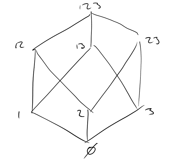
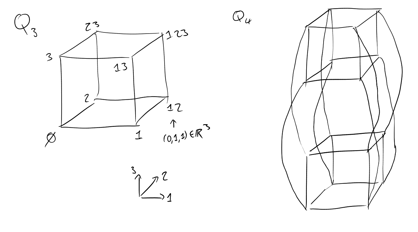
Definition 2 (Discrete cube). Make $P (X)$ into a graph by joining $A$ and $B$ if $| A Δ B | = 1$ , i.e. if $A = B \cup {i}$ for some $i$ , or vice versa. We call this ths discrete cube $Q_{n}$ (if $X = [n]$ ).

Example. $Q_{3}$ :

In general:

Alternatively, can view $Q_{n}$ as an $n$ -dimensional unit cube ${0, 1}^{n}$ , by identifying e.g. ${1, 3}$ with $1010000 \dots 0$ (i.e. identify $A$ with $𝟙_{A}$ , the characteristic function of $A$ ).

Example.

Definition 3 (Chain). Say $A \subset P (X)$ is a chain if $\forall A, B \in A$ , either $A \subset B$ or $B \subset A$ .

Example. For example,

A = {23, 12357, 123567}

is a chain.

Definition 4 (Antichain). Say $A$ is an antichain if $\forall A, B \in A$ , $A \neq B$ , we have $A ⁄ \subset B$ .

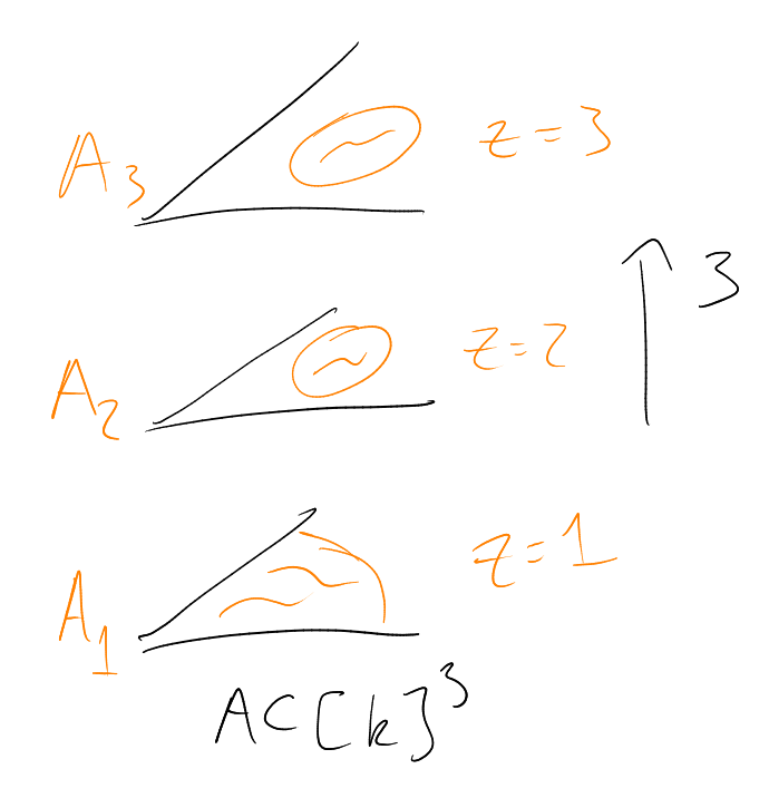
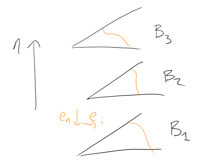
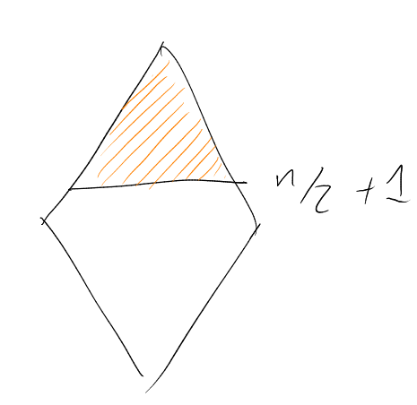
How large can a chain be? Can achieve $| A | = n + 1$ , for example using

A = {\emptyset, 1, 12, 123, \dots, [n]} .

Cannot beat this: for each $0 \leq r \leq n$ , $A$ contains $\leq 1$ $r$ -set.

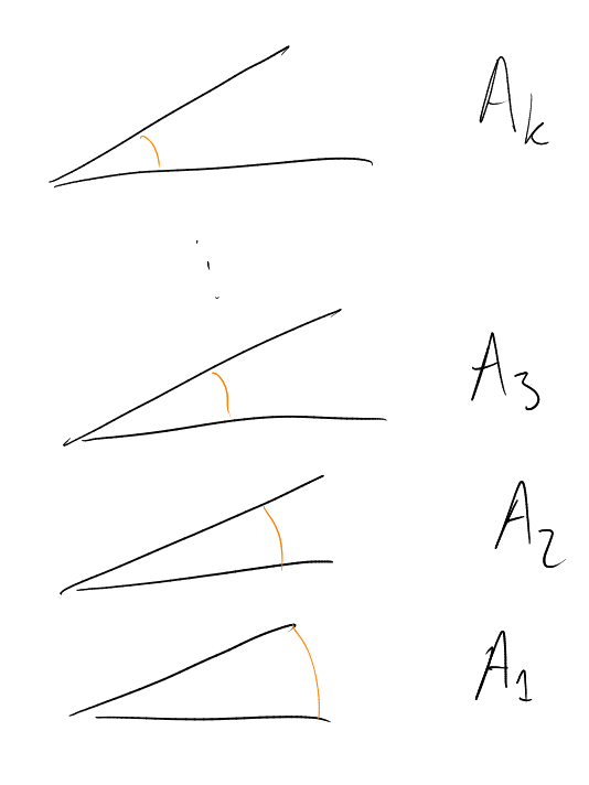
How large can an antichain be? Can achieve $| A | = n$ , for example $A = {1, 2, \dots, n}$ . More generally, can take $A = X^{(r)}$ , for any $r$ – best out of these is $X^{(⌊ \frac{n}{2} ⌋)}$ .

Can we beat this?

Theorem 5 (Sperner’s Lemma). Assuming that:

$A \subset P (X)$ is an antichain

Then

| A | \leq (\binom{n}{⌊ \frac{n}{2} ⌋})

Idea: Motivated by “a chain meets each layer in $\leq 1$ point, because a layer is an antichain”, we will try to decompose the cube into chains.

Proof. We’ll decompose $P (X)$ into $(\binom{n}{\frac{1}{2} n})$ chains – then done. To achieve this, it is sufficient to find:

(i) For each $r < \frac{n}{2}$ , a matching from $X^{(r)}$ to $X^{(r + 1)}$ (recall that a matching here means a set of disjoint edges, one for each point in $X^{(r)}$ ).
(ii) For each $r \geq \frac{n}{2}$ , a matching from $X^{(r)}$ to $^{(r - 1)}$ .

We then put these together to form our chains, each passing through $X^{(⌊ \frac{n}{2} ⌋)}$ .

By taking complements, it is enough to prove (i).

Let $G$ be the (bipartite) subgraph of $Q_{n}$ spanned by $X^{(r)} \cup X^{(r + 1)}$ : we seek a matching from $X^{(r)}$ to $X^{(r + 1)}$ . For any $S \subset X^{(r)}$ , the number of $S - Γ (S)$ edges in $G$ is $| S | (n - r)$ (counting from below) and $\leq | Γ (S) | (r + 1)$ (counting from above).

Hence, as $r < \frac{n}{2}$ ,

| Γ (S) | \geq \frac{| S | (n - r)}{r + 1} \geq | S | .

Thus by Hall’s Marriage theorem, there exists a matching. □

Equality in Sperner’s Lemma? Proof above tells us nothing.

Aim: If $A$ is an antichain then

\sum_{r = 0}^{n} \frac{| A \cap X^{(r)} |}{(\binom{n}{r})} \leq 1 .

“The percentages of each layer occupied add up to $\leq 1$ .”

Trivially implies Sperner’s Lemma (think about it).

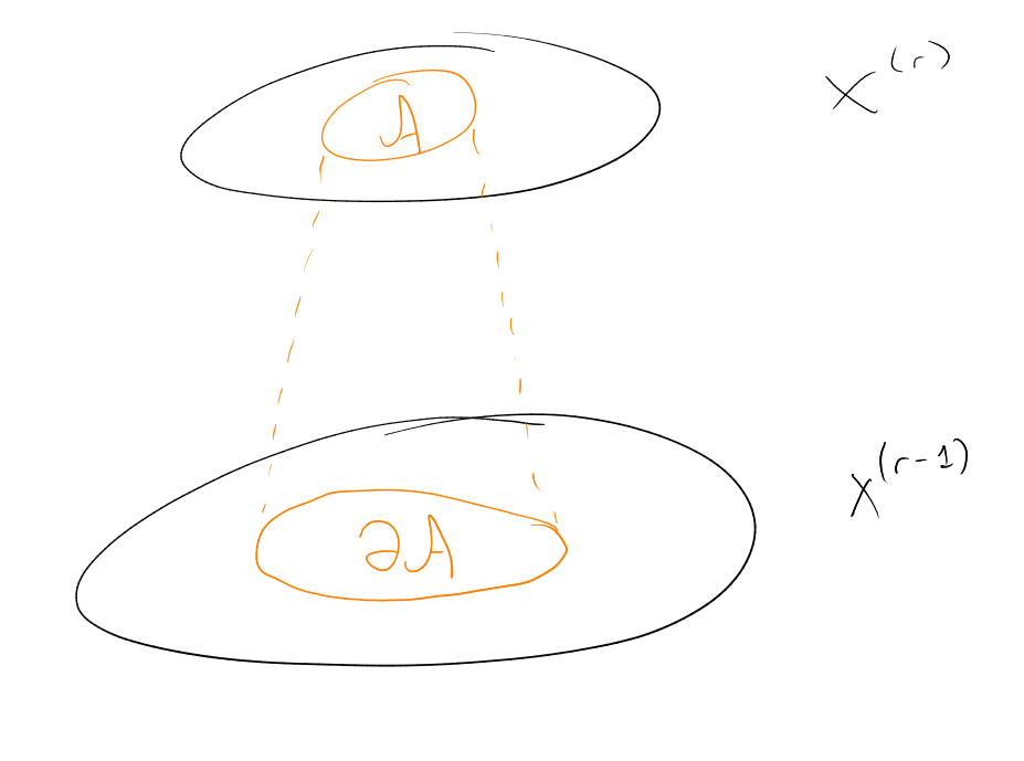
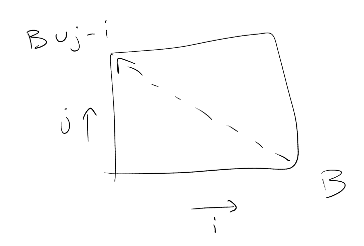
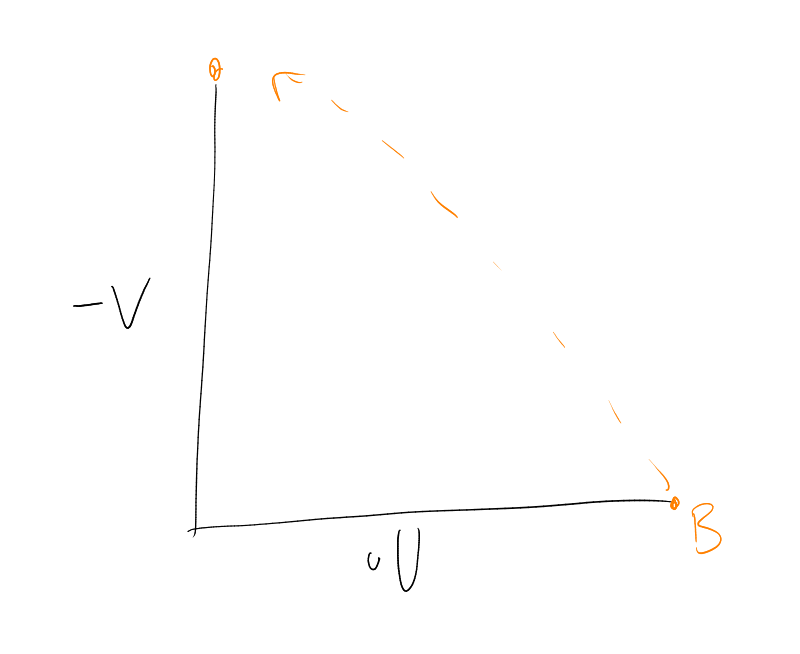
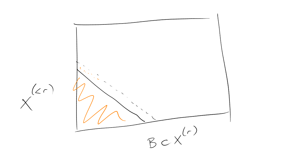
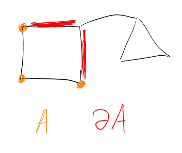
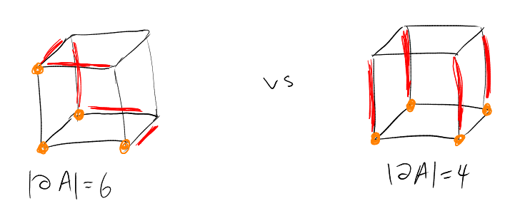
Definition 6 (Shadow). For $A \subset X^{(r)}$ ( $1 \leq r \leq n$ ), the shadow of $A$ is $\partial A = \partial^{-} A \subset X^{(r - 1)}$ defined by, $\partial A = {B \in X^{(r - 1)} : \exists A \in A, B \subset A}$ .

Example. If $A = {123, 124, 134, 137} \subset X^{(3)}$ , then $\partial A = {12, 13, 23, 14, 24, 34, 17, 37} \subset X^{(2)}$ .

Proposition 7 (Local LYM). Assuming that:

$A \subset X^{(r)}$
$1 \leq r \leq n$

Then

\frac{| \partial A |}{(\binom{n}{r - 1})} \geq \frac{| A |}{(\binom{n}{r})} .

“The fraction of the level occupied by $\partial A$ is $\geq$ the fraction for $A$ ”.

Remark. LYM = Lubell, Meshalkin, Yamamoto.

Proof. The number of $A - \partial A$ edges in $Q_{n}$ is $| A | r$ (counting from above) and is $\leq | \partial A | (n - r + 1)$ (counting from above). So

\frac{| \partial A |}{| A |} \geq \frac{r}{n - r + 1} .

But $\frac{(\binom{n}{r - 1})}{(\binom{n}{r})} = \frac{r}{n - r + 1}$ , so done. □

Equality in Local LYM? Must have that $\forall A \in A$ , $\forall i \in A$ , $\forall j \notin A$ have $A - {i} \cup {j} \in A$ . So $A = \emptyset$ or $X^{(r)}$ .

Theorem 8 (LYM Inequality). Assuming that:

$A \subset P (X)$ is an antichain

Then

\sum_{r = 0}^{n} \frac{| A \cap X^{(r)} |}{(\binom{n}{r})} \leq 1 .

Notation. We will now start writing $A_{r}$ for $A \cap X^{(r)}$ .

Proof 1. “Bubble down with Local LYM”.

Have $\frac{| A_{n} |}{(\binom{n}{n})} \leq 1$ . Now, $\partial A_{n}$ and $A_{n - 1}$ disjoint (as $A$ is an antichain), so

\frac{| \partial A_{n} |}{(\binom{n}{n - 1})} + \frac{| A_{n - 1} |}{(\binom{n}{n - 1})} = \frac{| \partial A_{n} \cup A_{n - 1}}{(\binom{n}{n - 1})} \leq 1,

whence

\frac{| A_{n} |}{(\binom{n}{n})} + \frac{| A_{n - 1} |}{(\binom{n}{n - 1})} \leq 1

by Local LYM.

Now, note $\partial (\partial A_{n} \cup A_{n - 1})$ is disjoint from $A_{n - 2}$ (since $A$ is an antichain), so

\frac{| \partial (\partial A_{n} \cup A_{n - 1}) |}{(\binom{n}{n - 2})} + \frac{| A_{n - 2} |}{(\binom{n}{n - 2})} \leq 1,

whence

\frac{| \partial A_{n} \cup A_{n - 1} |}{(\binom{n}{n - 1})} + \frac{| A_{n - 2} |}{(\binom{n}{n - 2})} .

(Local LYM) so

\frac{| A_{n} |}{(\binom{n}{n})} + \frac{| A_{n - 1} |}{(\binom{n}{n - 1})} + \frac{| A_{n - 2} |}{(\binom{n}{n - 2})} \leq 1 .

Continue inductively. □

Equality in LYM Inequality? Must have had equality in each use of Local LYM. Hence equality in LYM Inequality needs: max $r$ with $A_{r} \neq \emptyset$ has $A_{r} = X^{(r)}$ .

So: equality in Local LYM $⟺$ $A = X^{(r)}$ for some $r$ .

Hence: equality in Sperner’s Lemma if and only if $A = X^{(r)} \frac{n}{2}$ (if $n$ even), and $A = X^{(⌊ \frac{n}{2} ⌋)}$ or $A = X^{(⌈ \frac{n}{2} ⌉)}$ .

Proof 2. Choose, uniformly at random, a maximal chain $C$ (i.e. $C_{0} \subset C_{1} \subset C_{2} \subset \dots \subset C_{n}$ , with $| C_{r} | = r$ for all $r$ ).

For any $r$ -set $A$ , $ℙ (A \in C) = \frac{1}{(\binom{n}{r})}$ (all $r$ -sets are equally likely). So $ℙ (C meets A_{r}) = \frac{| A_{r} |}{(\binom{n}{r})}$ (as events are disjoint) and hence

1 \geq ℙ (C meets A) = \sum_{r = 0}^{n} \frac{| A_{r} |}{(\binom{n}{r})} . □

Equivalently: (if you want to lose the intuition about how this works) then: $#maximal chains = n!$ , and $#through any fixed r -set = r! (n - r)!$ , hence

\sum_{r} | A_{r} | r! (n - r)! \leq n! .

1.1 Shadows

For $A \subset X^{(r)}$ , know $| \partial A | \frac{r}{n - r + 1}$ . Equality is rare – only for $A = \emptyset$ or $X^{(r)}$ . What happens in between?

In other words, given $| A |$ , how should we choose $A \subset X^{(r)}$ to minimise $| \partial A |$ ?

Believable that if $| A | = (\binom{k}{r})$ then we sholud take $A = {[k]}^{(r)}$ .

What if $(\binom{k}{r}) < | A | < (\binom{k + 1}{r})$ ?

Believable that should take ${[k]}^{(r)}$ plus some $r$ -sets in ${[k + 1]}^{(r)}$ . For example, for $A \subset X^{(r)}$ with $| A | = (\binom{8}{3}) + (\binom{4}{2})$ , take $A = {[8]}^{(3)} \cup {9 \cup B : B \in {[4]}^{(2)}}$ .

1.2 Two total orders on $X^{(r)}$

Let $A$ and $B$ be distinct $r$ -sets: say $A = a_{1}, \dots, a_{r}$ , $B = b_{1}, \dots, b_{r}$ where $a_{1} < \dots < a_{r}$ and $b_{1} < \dots < b_{r}$ .

Say that $A < B$ in the lexicographic (or lex) ordering if for some $j$ we have $a_{i} = b_{i}$ for $i < j$ and $a_{j} < b_{j}$ .

Slogan: “Use small elements” (“dictionary order”).

Example. lexicographic on ${[4]}^{(2)}$ : $12, 13, 14, 23, 24, 34$ .

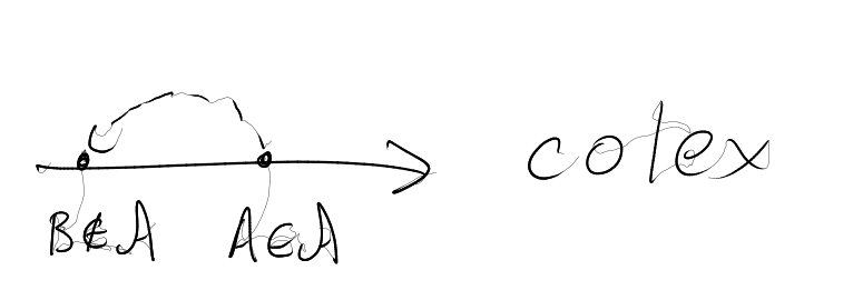
lexicographic on ${[6]}^{(3)}$ : $123, 124, 125, 126, 134, 135, 136, 145, 146, 156, 234, 235, 236, 245, 256, 345$ , $346, 356, 456$ .

Say that $A < B$ in the colexicographic (or colex) ordering if for some $j$ we have $a_{i} = b_{i}$ for all $i > j$ and $a_{j} < b_{j}$ .

Slogan: “Avoid large elements” (note that this is not quite the same as “use small elements”, which is what we had before).

Example. colexicographic on ${[4]}^{(2)}$ : $12, 13, 23, 14, 24, 34$ .

colexicographic on ${[6]}^{(3)}$ : $123, 124, 134, 234, 125, 135, 235, 145, 245, 345, 126, 136, 236, 146, 246, 346$ , $156, 256, 356, 456$ .

Note that, in colexicographic, ${[n - 1]}^{(r)}$ is an initial segment (first $t$ elements, for some $t$ ) of ${[n]}^{(r)}$ .

This is false for lex.

So we could view colexicographic as an enumeration of $ℕ^{(r)}$ .

Remark. $A < B$ in colexicographic if and only if $A^{c} < B^{c}$ in “lexicographic with ground set order reversed”.

Aim: colexicographic initial segments are best for $\partial$ , i.e. if $A \subset X^{(r)}$ and $C \subset X^{(r)}$ is the initial segment of colexicographic with $| C | = | A |$ , then $| \partial C | \leq | \partial A |$ .

In particular, $| A | = (\binom{k}{r}) ⟹ | \partial A | \geq (\binom{k}{r - 1})$ .

1.3 Compressions

Idea: try to transform $A \subset X^{(r)}$ into some $A^{'} \subset X^{(r)}$ such that:

(i) $| A^{'} | = | A |$ .
(ii) $| \partial A^{'} | \leq | \partial A |$ .
(iii) $A^{'}$ looks more like’ $C$ than $A$ did.

Ideally, we’d like a family of such ‘compressions’: $A \to A^{'} \to A^{″} \to A^{‴} \to \dots \to B$ such that either $B = C$ or $B$ is so similar to $C$ that we can directly check that $| \partial B | \geq | \partial C |$ .

“colexicographic prefers 1 to 2” inspires:

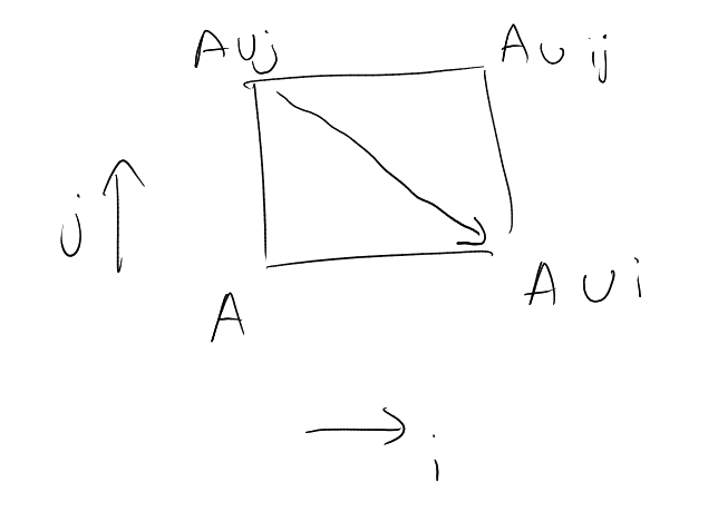
Definition 9 ( $i j$ -compression). Fix $1 \leq i < j \leq n$ . The $i j$ -compression $C_{i j}$ is defined as follows:

For $A \in X^{(r)}$ , set

C_{i j} (A) = {\begin{matrix} A \cup i - j & if j \in A, i \notin A \\ A & otherwise \end{matrix},

and for $A \subset X^{(r)}$ , set

C_{i j} (A) = {C_{i j} (A) : A \in A} \cup {A \in A : C_{i j} (A) \in A} .

Note that the second part of the union in $C_{i j} (A)$ is because we need to make sure that we “replace $j$ by $i$ where possible”.

Example. If $A = {123, 134, 234, 235, 146, 567}$ then $C_{12} (A) = {123, 134, 234, 135, 146, 567}$ .

So $C_{i j} (A) \subset X^{(r)}$ , and $| C_{i j} (A) | = | A |$ .

Say $A$ is $i j$ -compressed if $C_{i j} (A) = A$ .

Lemma 10. Assuming that:

$A \subset X^{(r)}$
$1 \leq i < j \leq n$

Then

| \partial C_{i j} (A) | \leq | \partial A |

Proof. Write $A^{'}$ for $C_{i j} (A)$ . Let $B \in \partial A^{'} - \partial A$ . We’ll show that $i \in B$ , $j \notin B$ and $B \cup j - i \in \partial A - \partial A^{'}$ . [Then done].

Have $B \cup x \in A^{'}$ for some $x$ , with $B \cup x \notin A$ (as $B \notin \partial A$ ). So $i \in B \cup x$ , $j \notin B \cup x$ , and $(B \cup x) \cup j - i \in A$ .

Cannot have $x = i$ , else $(B \cup x) \cup j - i = B \cup j$ , giving $B \in \partial A$ , contradiction.

Hence we have $i \in B$ , $j \notin B$ .

Also, $B \cup j - i \in \partial A$ , since $(B \cup x) \cup j - i \in A$ .

Suppose $B \cup j - i \in \partial A^{'}$ : so $(B \cup j - i) \cup y \in A^{'}$ for some $y$ . Cannot have $y = i$ , else $B \cup j \in A^{'}$ – so $B \cup j \in A$ (as $j \in B \cup j$ ), contradicting $B \notin \partial A$ . Hence $j \in (B \cup j - i) \cup y$ and $i \notin (B \cup j - i) \cup y$ .

Whence both $(B \cup j - i) \cup y$ and $B \cup y$ belong to $A$ (by definition of $A^{'}$ ), contradicting $B \notin \partial A$ . □

Remark. Actually showed that $\partial C_{i j} (A) \subset C_{i j} \partial A$ .

Definition 11 (Left-compressed). Say $A \subset X^{(r)}$ is left-compressed if $C_{i j} (A) = A$ for all $i < j$ .

Corollary 12. Let $A \subset X^{(r)}$ . Then there exists a left-compressed $B \subset X^{(r)}$ with $| B | = | A |$ and $| \partial B | \leq | \partial A |$ .

Proof. Define a sequence $A_{0}, A_{1}, \dots$ as follows. Set $A_{0} = A$ . Having defined $A_{0}, \dots, A_{k}$ , if $A_{k}$ left-compressed then stop the sequence with $A_{k}$ .

If not, choose $i < j$ such that $A_{k}$ is not $i j$ -compression, and set $A_{k + 1} = C_{i j} (A_{k})$ .

This must terminate, because for example $\sum_{A \in A_{k}} \sum_{i \in A}$ is strictly decreasing in $k$ .

Final term $B = A_{k}$ satisfies $| B | = | A |$ , and $| \partial B | \leq | \partial A |$ (by Lemma 10) □

Remark.

(1) Or: among all $B \subset X^{(r)}$ with $| B | = | A |$ and $| \partial B | \leq | \partial A |$ , choose one with minimal $\sum_{A \in B} \sum_{i \in A} i$ .
(2) Can choose order of the $C_{i j}$ so that no $C_{i j}$ applied twice.
(3) Any initial segment of colexicographic is left-compressed. Converse false, for example ${123, 124, 125, 126}$ (initial segment of lexicographic).

These compressions only encode the idea “colexicographic prefers $i$ to $j$ ( $i < j$ )”, but this is also true for lexicographic.

So we try to come up with more compressions that encode more of what colexicographic likes.

“colexicographic prefers $23$ to $14$ ” inspires:

Definition 13 ( $U V$ -compression). Let $U, V \subset X$ with $| U | = | V |$ , $U \cap V = \emptyset$ and $\max V > \max U$ . We define the $U V$ -compression as follows: for $A \subset X$ ,

C_{U V} (A) = {\begin{matrix} A \cup U - V & if V \subset A, U \cap A = \emptyset \\ A & otherwise \end{matrix},

and for $A \subset X^{(r)}$ , set

C_{U V} (A) = {C_{U V} (A) : A \in A} \cup {A \in A : C_{U V} \in A} .

Example. If

A = {123, 124, 147, 237, 238, 149},

then

C_{23, 14} (A) = {123, 124, 147, 237, 238, 239} .

So $C_{U V} (A) \subset X^{(r)}$ , and $| C_{U V} (A) | = | A |$ .

Say $A$ is $U V$ -compressed if $C_{U V} (A) = A$ .

Sadly, we can have $| \partial C_{U V} (A) | > | \partial A |$ :

Example. $A = {147, 157}$ has $| \partial A | = 5$ , but $C_{23, 14} (A) = {237, 147}$ has $| \partial C_{23, 14} (A) | = 6$ .

Despite this, we at least we do have the following:

Lemma 14. Assuming that:

$A \subset X^{(r)}$ is $U V$ -compression for all $U, V$ with $| U | = | V |$ , $U \cap V = \emptyset$ , $\max V > \max U$

Then

A

is an initial segment of colexicographic.

Proof. Suppose not. So there exists $A, B \in X^{(r)}$ with $B < A$ , in colexicographic but $A \in A$ , $B \notin A$ .

Put $V = A ∖ B$ , $U = B ∖ A$ .

Then $| V | = | U |$ , and $U, V$ disjoint, and $\max V > \max U$ (since $\max (A Δ B) \in A$ , by definition of colexicographic).

So $C_{U V} (A) = B$ , contradicting $A$ is $U V$ -compression. □

Lemma 15. Assuming that:

$U, V \subset X$
$| U | = | V |$
$U \cap V = \emptyset$
$\max U < \max V$
$A \subset X^{(r)}$
$\forall u \in U \exists v \in V such that A is (U - u, V - v) -compressed (∗)$

Then

| \partial C_{U V} (A) | \leq | \partial A |

Proof. Let $A^{'} = C_{U V} (A)$ . For $B \in \partial A^{'} - \partial A$ , we’ll show $U \subset B$ , $V \cap B = \emptyset$ , and $B \cup V - U \in \partial A - \partial A^{'}$ . (Then done).

Have $B \cup x \in A^{'}$ for some $x$ , and $B \cup x \notin A$ , so $U \subset B \cup x$ , $V \cap (B \cup x) = \emptyset$ , and $(B \cup x) \cup V - U \in A$ (by definition of $C_{U V}$ ).

If $x \in U$ : there exists $y \in U$ such that $A$ is $(U - x, V - y)$ -compressed, so from $(B \cup x) \cup V - U \in A$ we have $B \cup y \in A$ – contradicting $B \notin \partial A$ , contradiction.

Thus $x \notin U$ , and so $U \subset B$ , $V \cap B = \emptyset$ . Certainly $B \cup V - U \in \partial A$ (because $(B \cup x) \cup V - U \in A$ ), so just need to show that $B \cup V - U \notin \partial A^{'}$ .

Suppose $B \cup V - U \in \partial A^{'}$ : so $(B \cup V - U) \cup w \in A^{'}$ , for some $w$ . Also have $(B \cup V - U) \cup w \in A$ (for example, as $V$ contained in it).

If $w \in U$ : know $A$ is $(U - w, V - z)$ -compressed for some $z \in V$ , so $B \cup z \in A$ – contradicting $B \notin \partial$ .

If $w \notin U$ : have $V \subset (B \cup V - U) \cup w$ , $U \cap ((B \cup V - U) \cup w) = \emptyset$ , so by definition of $C_{U V}$ we must have that both $(B \cup V - U) \cup w$ and $B \cup w \in A$ – contradicting $B \notin \partial A$ , a contradiction. □

Theorem 16 (Kruskal-Katona). Assuming that:

$A \subset X^{(r)}$ , $1 \leq r \leq n$
$C$ is the initial segment of colexicographic on $X^{(r)}$ with $| C | = | A |$

Then

| \partial C | \leq | \partial A |

. In particular: if

| A | = (\binom{k}{r})

, then

| \partial A | \geq (\binom{k}{r - 1})

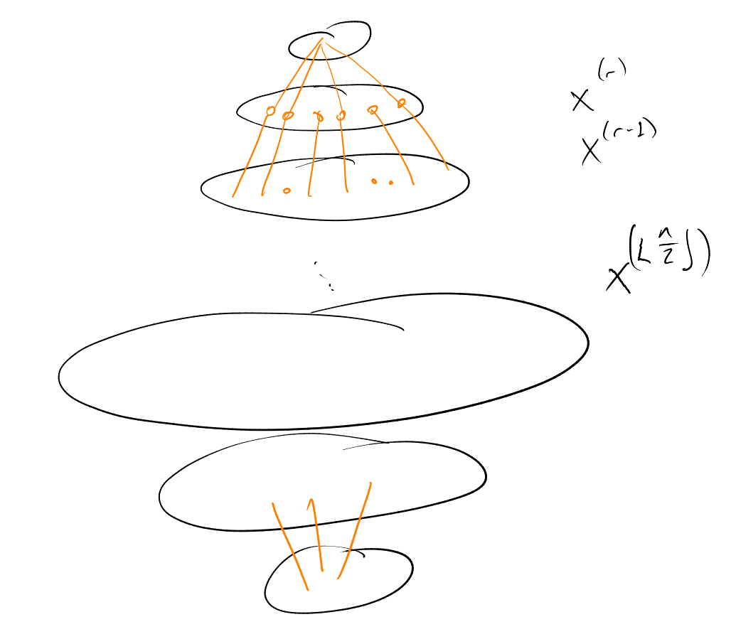
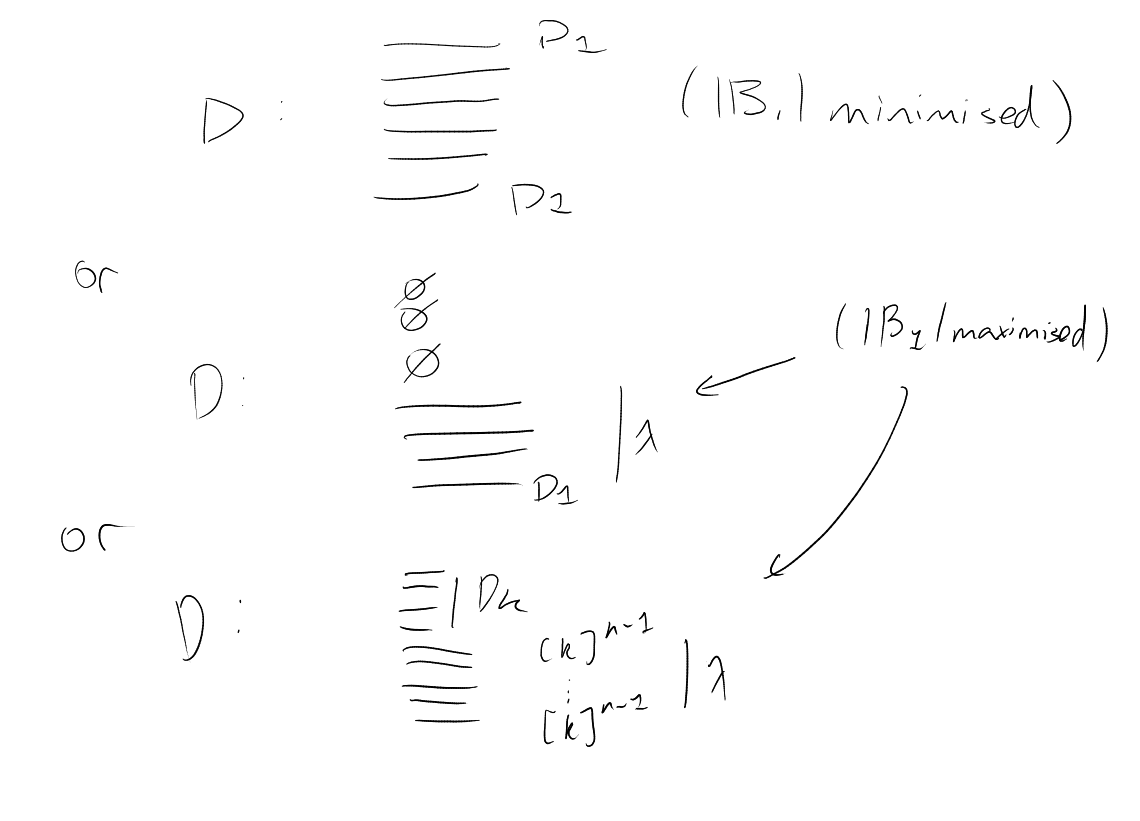
Proof. Let $Γ = {(U, V) : | U | = | V | > 0, U \cap V = \emptyset, \max U < \max V} \cup {(\emptyset, \emptyset)}$ . Define a sequence $A_{0}, A_{1}, \dots$ of set systems in $X^{(r)}$ as follows:

Set $A_{0} = A$ .
Having chosen $A_{0}, \dots, A_{k}$ , if $A_{k}$ is $U V$ -compressed for all $(U, V) \in Γ$ then stop. Otherwise, choose $U, V \in Γ$ with $| U | = | V | > 0$ minimal such that $A_{k}$ is not $U V$ -compressed.

Note that $\forall u \in U \exists v \in V$ such that $(U - u, V - v) \in Γ$ (namely, use $v = \min V$ ). So ( $*$ ) is satisfied.

So Lemma 15 tells us that $| \partial C_{U V} (A_{k}) | \leq | \partial A_{k} |$ .

Set $A_{k + 1} = C_{U V} (A_{k})$ , and continue.

Must terminate, as $\sum_{A \in A_{k}} \sum_{i \in A} 2^{i}$ is strictly decreasing. The final term $B = A_{k}$ satisfies $| B | = | A |$ , $| \partial B | \leq | \partial A |$ and is $U V$ -compressed for all $(U, V) \in Γ$ .

So $B = C$ by Lemma 14. □

Remark.

(1) Equivalently: if
$| A | = (\binom{k_{r}}{r}) + (\binom{k_{r - 1}}{r - 1}) + \dots + (\binom{k_{s}}{s}),$

where $k_{r} > k_{r - 1} > \dots > k_{s}$ , and $s \geq 1$ , then
$(\binom{| \partial A | \geq (\binom{k_{r}}{r - 1}) + (\binom{k_{r - 1}}{r - 2}) +}{+ (\binom{k_{s}}{s - 1}) .})$
(2) Equality in Kruskal-Katona? Can check that if $| A | = (\binom{k}{r})$ and $| \partial | = (\binom{k}{r - 1})$ (i.e. equality in a step of the proof of Kruskal-Katona), then $A = Y^{(r)}$ , for some $Y \subset X$ with $| Y | = k$ .
(3) However, not true in general that $| \partial A | = | \partial C |$ implies that $A$ is isomorphic to $C$ . (uset systems $A, B$ are isomorphic if there exists permutation of the ground set $X$ sending $A$ to $B$ ).

For $A \subset X^{(r)}$ , $0 \leq r \leq n$ , the upper shadow of $A$ is

\partial^{+} A = {A \cup x : A \in A, x \notin A} \subset X^{(r + 1)} .

Corollary 17. Let $A \subset X^{(r)}$ , where $0 \leq r \leq n$ , and let $C$ be the initial segment of lexicographic on $X^{(r)}$ with $| C | = | A |$ . Then $| \partial^{+} A | \geq | \partial^{+} C |$ .

Proof. From Kruskal-Katona, since $A < B$ in colexicographic if and only if $A^{c} < B^{c}$ in lexicographic with ground-set order reversed. □

Note that the shadow of an initial segment of colexicographic on $X^{(r)}$ is an initial segment of colexicographic on $X^{(r - 1)}$ – as if $C = {A \in X^{(r)} : A \leq a_{1} \dots a_{r} in colexicographic}$ then $\partial C = {B \in X^{(r - 1)} : B \leq a_{2} \dots a_{r} in colexicographic}$ .

This fact gives:

Corollary 18. Let $A \subset X^{(r)}$ , and $C$ is the initial segment of colexicographic on $X^{(r)}$ with $| C | = | A |$ . Then $| \partial^{t} C | \leq | \partial^{t} A |$ for all $1 \leq t \leq r$ .

Proof. If $| \partial^{t} C \leq | \partial^{t} A |$ , then $| \partial^{t + 1} C | \leq | \partial^{t + 1} A |$ , because $\partial^{t} C$ is an initial segment of colexicographic. Done by induction. □

Note. If $| A | = (\binom{k}{r})$ , then $| \partial^{t} A | \geq (\binom{k}{r - t})$ .

Remark. Proof of Kruskal-Katona used Lemma 14 and Lemma 15, but not Lemma 10 or Corollary 12.

1.4 Intersecting Families

Say $A \subset P (X)$ intersecting if $A \cap B \neq \emptyset$ for all $A, B \in A$ .

How large can an intersecting family be? Can have $| A | = 2^{k - 1}$ , by taking $A = {A : 1 \in A}$ .

Proposition 19. Assuming that:

$A \subset P (X)$ be intersecting

Then

| A | \leq 2^{k - 1}

Proof. For any $A \subset X$ , at most one of $A, A^{c}$ can belong to $A$ . □

Note. Many other extremal examples. For example, for $n$ odd take ${A : | A | > \frac{k}{2}}$ .

What if $A \subset X^{(r)}$ ?

If $r > \frac{n}{2}$ , take $A = X^{(r)}$ .

If $r = \frac{n}{2}$ : just choose one of $A, A^{c}$ for all $A \in X^{(r)}$ : gives $| A | = \frac{1}{2} (\binom{n}{r})$ .

So interesting case is $r < \frac{n}{2}$ .

Could try $A = {A \in X^{(r)} : 1 \in A}$ . Has size $(\binom{n - 1}{r - 1}) = \frac{r}{n} (\binom{n}{r})$ (while this identity can be verified by writing out factorials, a more useful way of observing it is by noting that $ℙ (random r -set contains 1) = \frac{r}{n}$ ).

Could also try $B = {A \in X^{(r)} : | A \cap {1, 2, 3} | \geq 2}$ .

Example. $n = 8$ , $r = 3$ . Then $| A | = (\binom{7}{2}) = 21$ and

| B | = \underset{| B \cap [3] | = 3}{\underset{⏟}{1}} + \underset{| B \cap [3] | = 2}{\underset{⏟}{(\binom{3}{2}) (\binom{5}{1})}} = 16 < 21 .

Theorem 20 (Erdos-Ko-Rado Theorem). Assuming that:

$A \subset X^{(r)}$ be intersecting, where $r < \frac{n}{2}$

Then

| A | \leq (\binom{n - 1}{r - 1})

Proof 1 (“Bubble down with Kruskal-Katona”). Note that $A \cap B \neq \emptyset ⟺ A ⁄ \subset B^{c}$ .

Let $\bar{A} = {A^{c} : A \in A} \subset X^{(n - r)}$ . Have $\partial^{n - 2 r} \bar{A}$ and $A$ are disjoint families of $r$ -sets.

Suppose $| A | > (\binom{n - 1}{r - 1})$ . Then $| \bar{A} | = | A | > (\binom{n - 1}{r - 1}) = (\binom{n - 1}{n - r})$ . Whence by Kruskal-Katona we have $| \partial^{n - 2 r} \bar{A} | \geq (\binom{n - 1}{r})$ .

So $| A | + | \partial^{n - 2 r} \bar{A} | > (\binom{n - 1}{r - 1}) + (\binom{n - 1}{r}) = (\binom{n}{r})$ , a contradiction. □

Remark. Calculation at the end had to give the right answer, as the $\partial$ calculations would all be exact if $A = {A \in X^{(r)} : 1 \in A}$ .

Proof 2. Pick a cyclic ordering of $[n]$ i.e. a bijection $c : [n] \to ℤ_{n}$ .

How many sets in $A$ are intervals ( $r$ consecutive elements) in this ordering?

Answer: $\leq r$ . Because say $C_{1}, \dots, C_{r} \in A$ . Then for each $2 \leq i \leq 1$ , at most one of the two intervals $C_{i} C_{i + 1} \dots C_{i + r - 1}$ and $C_{i - r} C_{i - r + 1} \dots C_{i - 1}$ can belong to $A$ (subscrpits are modulo $n$ ).

For each $r$ -set $A$ , in how many of the $n!$ cyclic orderings is it an interval?

Answer: $n r! (n - r)!$ ( $n =$ where, $r! =$ order inside $A$ , $(n - r)! =$ order outside $A$ ).

Hence $A | n r! (n - r)! \leq n! r$ , i.e. $| A | \leq \frac{n! r}{n r! (n - r)!} = (\binom{n - 1}{r - 1})$ . □

Remark.

(1) Numbers had to work out, given that we get equality $A = {A \in X^{(r)} : 1 \in A}$ .
(2) Equivalently, we are double-counting the edges in the bipartite graph, with vertex classes $A$ and all cycling orderings, with $A$ joined to $c$ if $A$ is an interval in $c$ .
(3) This method is caled averaging or Katona’s method.
(4) Equality in Erdos-Ko-Rado Theorem? Our example is actually unique – if $A \subset X^{(r)}$ is intersecting and $| A | = (\binom{n - 1}{r - 1})$ , then $A = {A \in X^{(r)} : i \in A}$ for some $1 \leq i \leq n$ .
Can get this from Proof 1 (and equality in Kruskal-Katona) or from Proof 2 (with a bit of care).

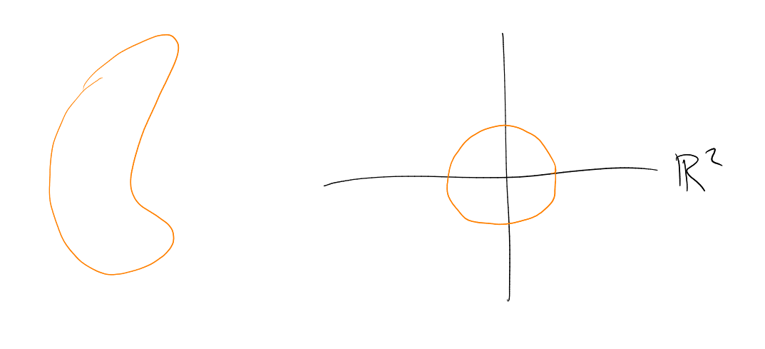
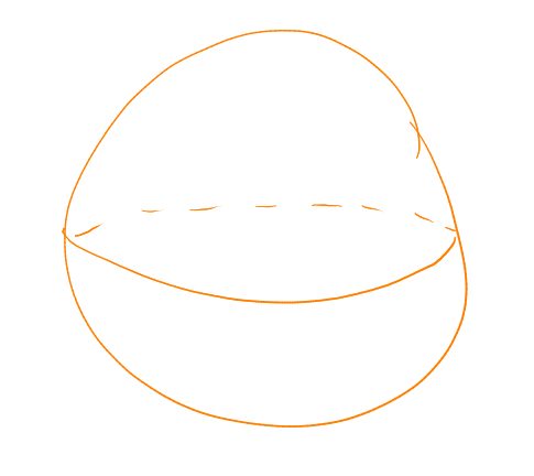
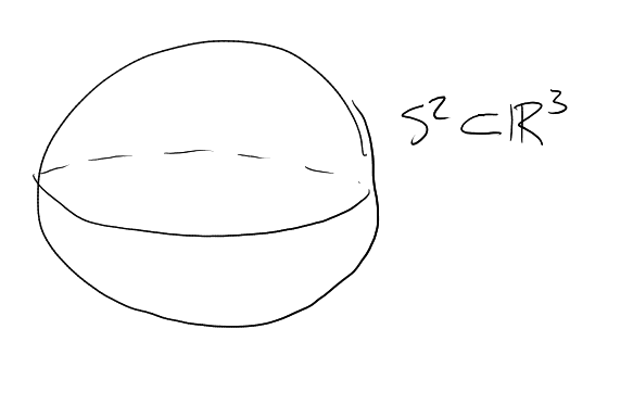
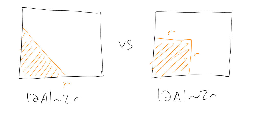
2 Isoperimetric Inequalities

“How do we minimise the boundary of a set of given size?”

Example. Among all subsets of $ℝ^{2}$ of given area, the disc minimises the perimeter.

Among all subsets of $ℝ^{3}$ of given volume, the solid sphere minimises the surface area.

Among all subsets of $S^{2}$ of given surface area, the circular arc has the smallest perimeter.

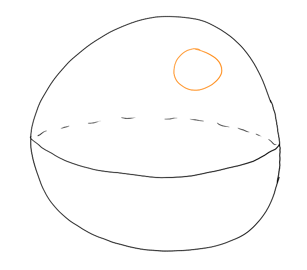
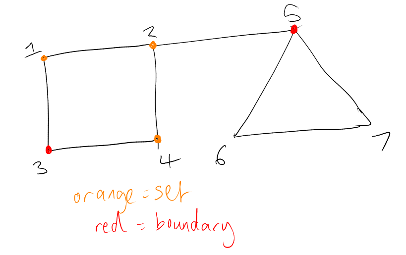
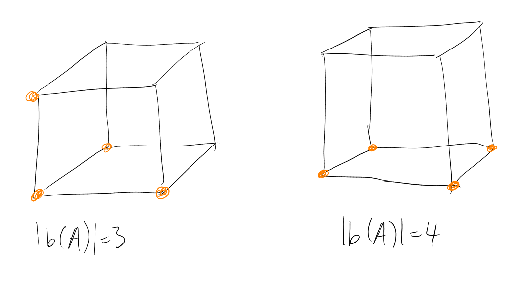
Definition (Boundary in a graph). For a set $A$ of vertices of a graph $G$ , the boundary of $A$ is

b (A) = {x \in G : x \notin A, x y \in E for some y \in A} .

Example. Here, if $A = {1, 2, 4}$ , then $b (A) = {3, 5}$ .

Definition (Isoperimetric inequality). An isoperimetric inequality on $G$ is an inequality of the form

| b (A) | \geq f (| A |) \forall A \subset G,

for some function $f$ .

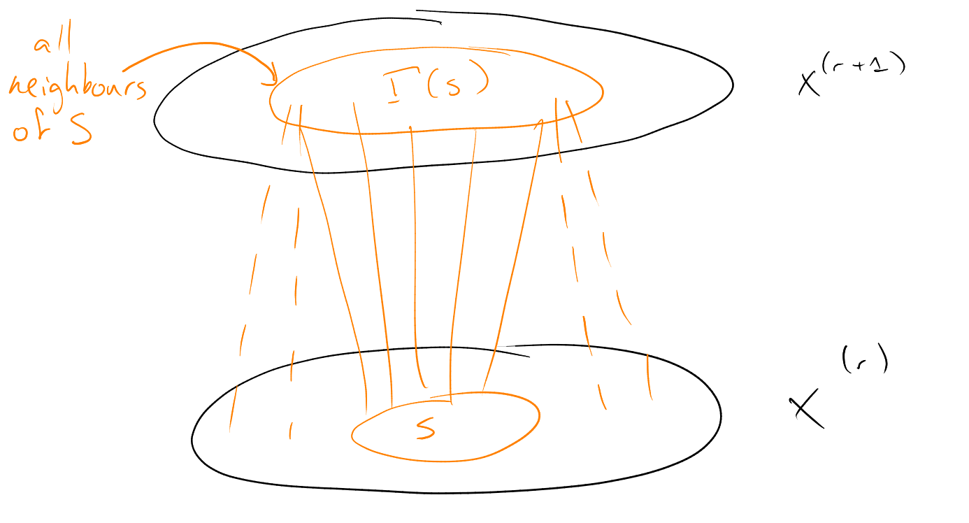
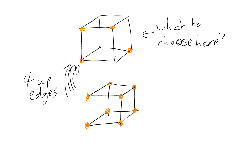
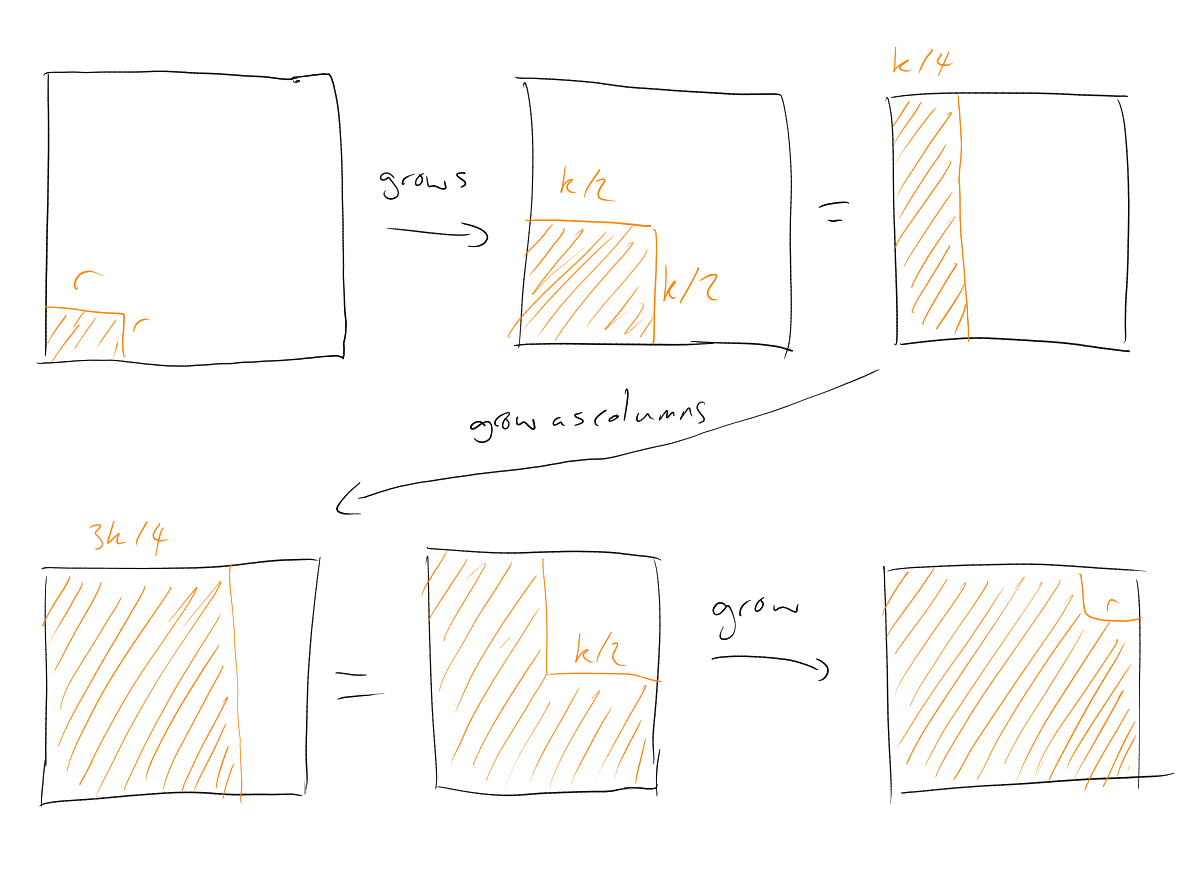
Definition (Neighbourhood). Often simpler to look at the neighbourhood of $A$ : $N (A) = A \cup b (A)$ . So

N (A) = {x \in G : d (x, A) \leq 1} .

A good example for $A$ might be a ball $B (x, r) = {y \in G : d (x, y) \leq r}$ . What happens for $Q_{n}$ ?

Example. $| A | = 4$ in $Q_{3}$ .

Good guess that balls are best, i.e. sets of the form $B (\emptyset, r) = X^{(\leq r)} = X^{(0)} \cup X^{(1)} \cup \dots \cup X^{(r)}$ .

What if $| X^{(\leq r)} | < | A | < | X^{(r + 1)} |$ ?

Guess: take $A$ with $X^{(\leq r)} < A < X^{(\leq r + 1)}$ . If $A = X^{(\leq r)} \cup B$ , where $B \subset X^{(r + 1)}$ , then $b (A) = (X^{(r + 1)} - B) \cup \partial^{+} B$ . So we’d take $B$ to be an initial segment of lexicographic (by Kruskal-Katona).

This suggests...

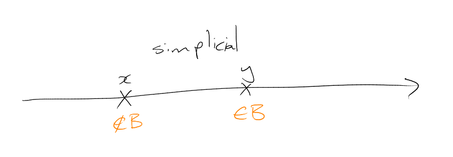
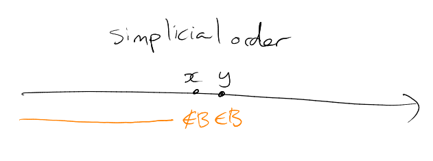
In the simplicial ordering on $P (X)$ , we set $x < y$ if either $| x | < | y |$ or $| x | = | y |$ and $x < y$ in lexicographic.

Aim: initial segments of simplicial ordering minimise the boundary.

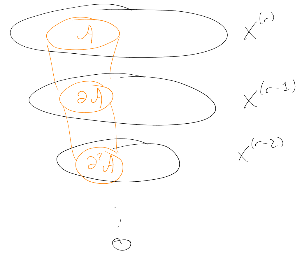
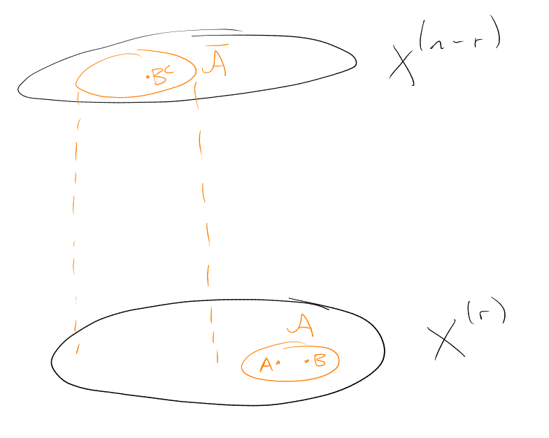
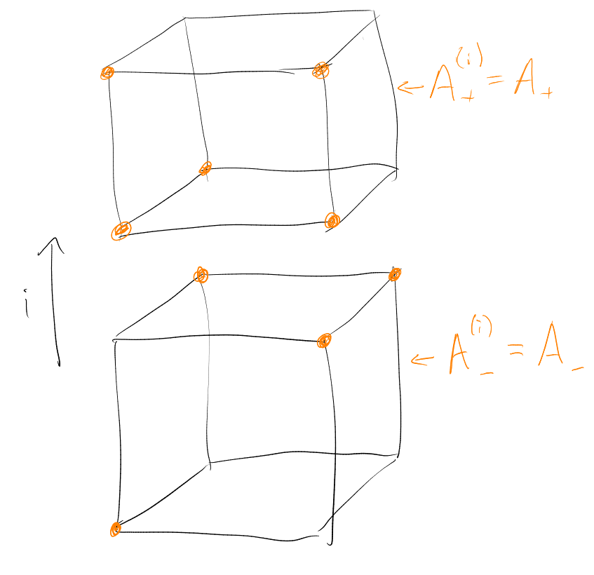
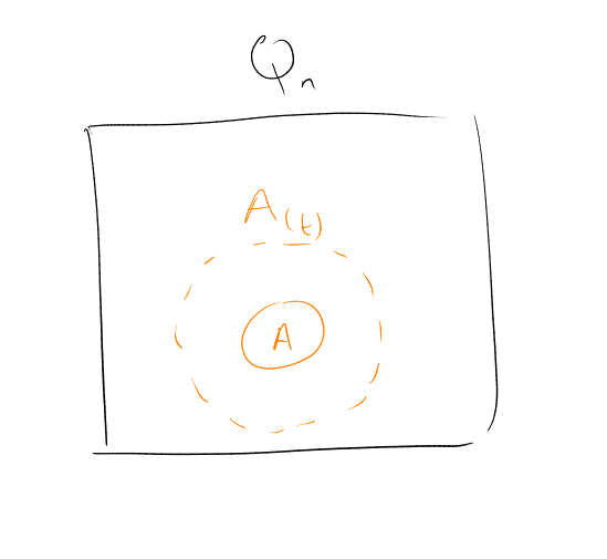
Definition ( $i$ -sections). For $A \subset P (X)$ and $1 \leq i \leq n$ , the $i$ -sections of $A$ are the families $A_{-}^{(i)}, A_{+}^{(i)} \subset P (X - i)$ given by:

\begin{array}{l} A_{-}^{(i)} & = {x \in A : i \notin x} \\ A_{+}^{(i)} & = {x - i : x \in A, i \in x} \end{array}

The $i$ -compression of $A$ in the family $C_{i} (A) \subset P (X)$ given by:

${(C_{i} (A))}_{-}^{(i)}$ is the first $| A_{-}^{(i)} |$ elements of simplicial ordering on $P (X - i)$
${(C_{i} (A))}_{+}^{(i)}$ is the first $| A_{+}^{(i)} |$ elements of simplicial ordering on $P (X - i)$

Example.

Certainly $| C_{i} (A) | = | A |$ . Say $A$ is $i$ -compressed if $C_{i} (A) = A$ . Also, $C_{i} (A)$ “looks more like” a Hamming ball than $A$ does.

Here, a Hamming ball is a family $A$ with $X^{(\leq r)} \subset A \subset X^{(\leq r + 1)}$ , for some $r$ .

Theorem 1 (Harper’s Theorem). Assuming that:

$A \subset Q_{n}$
$C$ the initial segment of simplicial ordering with $| C | = | A |$

Then

| N (A) | \geq | N (C) |

. In particular, if

| A | = \sum_{i = 0}^{r} (\binom{n}{i})

then

| N (A) | \geq \sum_{i = 0}^{r + 1} (\binom{n}{i})

Remark.

(1) If we knew $A$ was a Hamming ball, then we would be done by Kruskal-Katona.
(2) Conversely, Harper’s Theorem implies Kruskal-Katona: given $B \subset X^{(r)}$ , then apply Harper’s Theorem to $A = X^{(\leq r - 1)} \cup B$ .

Proof. Induction on $n$ : $n = 1$ is trivial.

Given $n > 1$ , and $A \subset Q_{n}$ , and $1 \leq i \leq n$ .

Claim: $| N (C_{i} (A)) | \leq | N (A) |$ .

Proof of claim: Write $B$ for $C_{i} (A)$ . We have

\begin{array}{l} N {(A)}_{-} & = N (A_{-}) \cup A_{+} \\ N {(A)}_{+} & = N (A_{+}) \cup A_{-} \end{array}

and of course

\begin{array}{l} N {(B)}_{-} & = N (B_{-}) \cup B_{+} \\ N {(B)}_{+} & = N (B_{+}) \cup B_{-} \end{array}

Now, $| B_{+} | = | A_{+} |$ and $| N (B_{-}) | \leq | N (A_{-}) |$ (by the induction hypothesis). But $B_{+}$ is an initial segment of simplicial ordering, and $N (B_{-})$ is an initial segment of simplicial ordering (as neighbourhood of initial segment is an initial segment).

So then $B_{+}$ and $N (B_{-})$ are nested (one conatined in the other). Hence $| N {(B)}_{-} | \leq | N {(A)}_{-} |$ . Similarly, $| N {(B)}_{+} | \leq | N {(A)}_{+} |$ .

Hence $| N (B) | \leq | N (A) |$ , which completes the proof of our claim. □

Define a sequence $A_{0}, A_{1}, \dots \subset Q_{n}$ as follows:

Set $A_{0} = A_{1}$ .
Having chosen $A_{0}, \dots, A_{k}$ : if $A_{k}$ is $i$ -compressed with $C_{i} (A_{k}) \neq A_{k}$ and set $A_{k + 1} = C_{i} (A_{k})$ – and continue.

Must terminate, because $\sum_{x \in A_{k}} (position of x in simplicial ordering)$ is strictly decresing.

The final family $B = A_{k}$ satisfies $| B | = | A |$ , $| N (B) | \leq | N (A) |$ , and is $i$ -compressed for all $i$ . Does $B$ $i$ -compressed for all $i$ imply that $B$ is an initial segment of simplicial ordering? (If yes, then $B = C$ and we are done).

Sadly, no. For example in $Q_{3}$ can take ${\emptyset, 1, 2, 12}$ :

However:

Lemma 2. Assuming that:

$B \subset Q_{n}$ is $i$ -compressed for all $i$
$B$ not an initial segment of the simplicial ordering

Then one of the following is true:

either $n$ is odd, say $n = 2 k + 1$ , and $B = X^{(\leq k)} - {k + 2, k + 3, \dots, 2 k + 1} \cup {1, 2, \dots, k + 1}$
or $n$ is even, say $n = 2 k$ , and $B = X^{(< k)} \cup {x \in X^{(k)} : 1 \in x} - {1, k + 2, k + 3, \dots, 2 k} \cup {2, 3, 4, \dots, k + 1}$ .

For the even case: “Remove the last $k$ -set with $1$ , and add the first $k$ -set without $1$ .”

After we prove this, we will have solved our problem, as in each case we certainly have $| N (B) | \geq | N (C) |$ .

Proof. Since $B$ is not an initial segment of simplicial ordering, there exists $x < y$ (in simplicial ordering) with $x \notin B$ , $y \in B$ .

For each $1 \leq i \leq n$ : cannot have $i \in x$ , $i \in y$ (as $B$ is $i$ -compressed). Also cannot have $i \notin x$ , $i \notin y$ for the same reason.

So $x = y^{c}$ .

Thus: for each $y \in B$ , there exists at most one earlier $x$ with $x \notin B$ (namely $x = y^{c}$ ). Similarly, for each $x \notin B$ there is at most one later $y$ with $y \in B$ (namely $y = x^{c}$ ).

So $B = {z : z \leq y} - {x}$ , with $x$ the predessor of $y$ and $x = y^{c}$ .

Hence if $n = 2 k + 1$ then $x$ is the last $k$ -set, and if $n = 2 k$ then $x$ is the last $k$ -set with $1$ . □

Proof of Theorem 1. Done by above. □

Remark.

(1) Can also prove Harper’s Theorem $U V$ -compressions.
(2) Can also prove Kruskal-Katona using these ‘codimension $1$ ’ compressions.

For $A \subset Q_{n}$ and $t = 1, 2, 3, \dots$ , the $t$ -neighbourhood of $A$ is $A_{(t)} = N^{t} (A) = {x \in Q_{n} : d (x, A) \leq t}$ .

Corollary 3. Let $A \subset Q_{n}$ with $| A | \geq \sum_{i = 0}^{r} (\binom{n}{i})$ . Then

| A_{(t)} | \geq \sum_{i = 0}^{r + t} (\binom{n}{i})

for all $t \leq n - r$ .

Proof. Theorem 1 with induction on $t$ . □

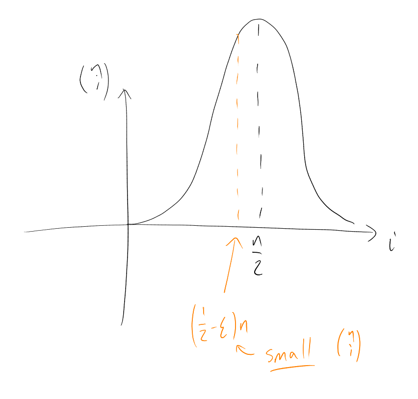
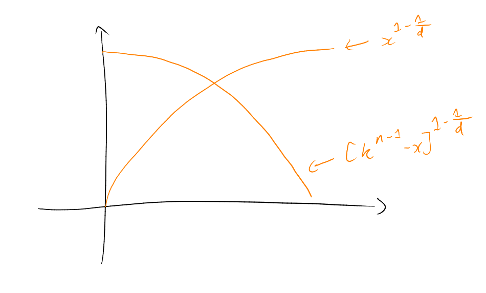
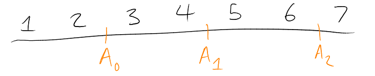
To get a feeling for the strength of Corollary 3, we’ll need some estimates on things like $\sum_{i = 0}^{r} (\binom{n}{i})$ .

“Going $𝜀 \sqrt{n}$ standard deviations away from the mean $\frac{n}{2}$ .”

Proposition 4. Assuming that:

$0 < 𝜀 < \frac{1}{4}$

Then

\sum_{i = 0}^{⌊ (\frac{1}{2} - 𝜀) n ⌋} (\binom{n}{i}) \leq \frac{1}{𝜀} e^{- \frac{𝜀^{2} n}{2}} \cdot 2^{n} .

“For $𝜀$ fixed, $n \to \infty$ , this is an exponentially small fraction of $2^{n}$ .”

Proof. For $i \leq ⌊ (\frac{1}{2} - 𝜀) n ⌋$ :

(\binom{n}{i}) = (\binom{n}{i}) \frac{i}{n - i + 1},

\frac{(\binom{n}{i - 1})}{(\binom{n}{i})} = \frac{i}{n - i + 1} \leq \frac{(\frac{1}{2} - 𝜀) n}{(\frac{1}{2} + 𝜀) n} = \frac{\frac{1}{2} - 𝜀}{\frac{1}{2} + 𝜀} = 1 - \frac{2 𝜀}{\frac{1}{2} + 𝜀} \leq 1 - 2 𝜀 .

Hence

\sum_{i = 0}^{⌊ (\frac{1}{2} - 𝜀) n ⌋} (\binom{n}{i}) \leq \frac{1}{2 𝜀} (\binom{n}{⌊ (\frac{1}{2} - 𝜀) n ⌋})

(sum of a geometric progression).

Same argument tells us that

\begin{array}{l} (\binom{n}{⌊ (\frac{1}{2} - 𝜀) n ⌋}) & \leq (\binom{n}{⌊ (\frac{1}{2} - \frac{𝜀}{2}) n ⌋}) {(1 - 2 \frac{𝜀}{2})}^{\frac{𝜀 n}{2} - 1} & -1 from the ⌊ ∙ ⌋ stuff \\ \leq 2^{n} \cdot 2 {(1 - 𝜀)}^{\frac{𝜀 n}{2}} \\ \leq 2^{n} \cdot 2 e^{- \frac{𝜀^{2} n}{2}} & as 1 - 𝜀 \leq e^{- 𝜀} \end{array}

Thus

\sum_{i = 0}^{⌊ (\frac{1}{2} - 𝜀) n ⌋} (\binom{n}{i}) \leq \frac{1}{2 𝜀} \cdot 2 e^{- \frac{𝜀^{2} n}{2}} \cdot 2^{n} . □

Theorem 5. Assuming that:

$0 < 𝜀 < \frac{1}{4}$
$A \subset Q_{n}$
$\frac{| A |}{2^{n}} \geq \frac{1}{2}$

Then

\frac{| A_{(𝜀 n)} |}{2^{n}} \geq 1 - \frac{2}{𝜀} e^{- \frac{𝜀^{2} n}{2}}

“ $\frac{1}{2}$ -sized sets have exponentially large $𝜀 n$ -neighbourhoods.”

Proof. Enough to show that if $𝜀 n$ an integer then

\frac{| A_{(𝜀 n)} |}{2^{n}} \geq 1 - \frac{1}{𝜀} e^{- \frac{𝜀^{2} n}{2}} .

Have $| A | \geq \sum_{i = 0}^{⌈ \frac{n}{2} - 1 ⌉} (\binom{n}{i})$ , so by Harper’s Theorem, we have $| A_{(𝜀 n)} | \geq \sum_{i = 0}^{⌈ \frac{n}{2} - 1 + 𝜀 n ⌉} (\binom{n}{i})$ , so

| A_{(𝜀 n)}^{c} | \leq \sum_{i = ⌈ \frac{n}{2} + 𝜀 n ⌉}^{n} (\binom{n}{i}) = \sum_{i = 0}^{⌊ \frac{n}{2} - 𝜀 n ⌋} (\binom{n}{i}) \leq \frac{1}{𝜀} e^{- \frac{𝜀^{2} n}{2}} 2^{n} . □

Remark. Same would show, for “small” sets:

\frac{| A |}{2^{n}} \geq \frac{2}{𝜀} e^{- \frac{𝜀^{2} n}{2}} ⟹ \frac{| A_{(2 𝜀 n)} |}{2^{n}} \geq 1 - \frac{2}{𝜀} e^{- \frac{𝜀^{2} n}{2}} .

2.1 Concentration of measure

Say $f : Q_{n} \to ℝ$ is Lipschitz if $| f (x) - f (y) | \leq 1$ for all $x, y$ adjacent.

For $f : Q_{n} \to ℝ$ , say $M \in ℝ$ is a Lévy mean or median of $f$ if

| {x \in Q_{n} : f (x) \leq M} | \geq 2^{n - 1}

and

| {x \in Q_{n} : f (x) \geq M} | \geq 2^{n - 1}

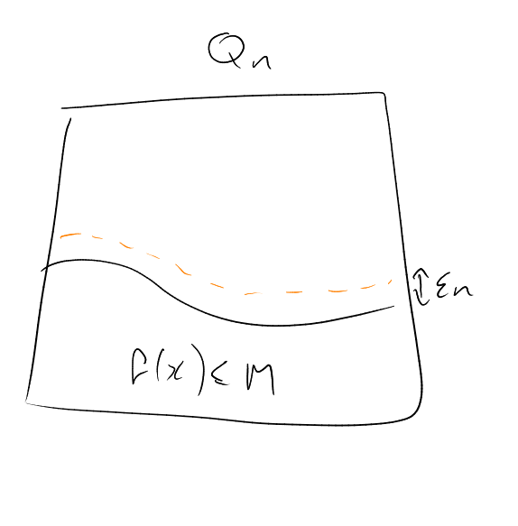
Now ready to show “every well-behaved function on the cube $Q_{n}$ is roughly constant nearly everywhere”.

Theorem 6. Assuming that:

$f : Q_{n} \to ℝ$ Lipschitz with median $M$

Then

\frac{| {x : | f (x) - M | \leq 𝜀 n} |}{2^{n}} \geq 1 - \frac{4}{𝜀} e^{- \frac{𝜀^{2} n}{2}}

for any $0 < 𝜀 < \frac{1}{4}$ .

Note. This is the “concentration of measure” phenomenon.

Proof. Let $A = {x : f (x) \leq M}$ . Then $\frac{| A |}{2^{n}} \geq \frac{1}{2}$ , so

\frac{| A_{(𝜀 n)} |}{2^{n}} \geq 1 - \frac{2}{𝜀} e^{- \frac{𝜀^{2} n}{2}} .

ut $f$ is Lipschitz, so $x \in A_{(𝜀 n)}$ implies $f (x) \leq M + 𝜀 n$ . Thus

\frac{| {x : f (x) \leq M + 𝜀 n} |}{2^{n}} \geq 1 - \frac{2}{𝜀} e^{- \frac{𝜀^{2} n}{2}} .

Similarly,

\frac{| {x : f (x) \geq M - 𝜀 n} |}{2^{n}} \geq 1 - \frac{2}{𝜀} e^{- \frac{𝜀^{2} n}{2}} .

Hence

\frac{| {x : M - 𝜀 n \leq f (x) \leq M + 𝜀 n} |}{2^{n}} \geq 1 - \frac{4}{𝜀} e^{- \frac{𝜀^{2} n}{2}} . □

Let $G$ be a graph of diameter $D$ ( $D = \max {f (x, y) : x, y \in G}$ ).

Definition ( $α (G, 𝜀)$ ). Write

α (G, 𝜀) = \max {1 - \frac{| A_{(𝜀 D)} |}{| G |} : A \subseteq G, \frac{| A |}{| G |} \geq \frac{1}{2}} .

So $α (G, 𝜀)$ small says “ $\frac{1}{2}$ -sized sets have large $𝜀 D$ -neighbourhoods”.

Definition (Levy family). Say a sequence of graphs is a Lévy family if $α (G_{n}, 𝜀) \to 0$ as $n \to \infty$ , for each $𝜀 > 0$ .

So Theorem 5 tells us that the sequence $(Q_{n})$ is a Lévy family – even a normal Lévy family, meaning $α (G_{n}, 𝜀)$ grows exponentially small in $n$ , for each $𝜀 > 0$ .

So have concentration of measure for any Lévy family.

Many naturally-occurring families of graphs are Lévy families.

Example. $(S_{n})$ , where $S_{n}$ is made into a graph by joining $σ$ to $σ^{'}$ if $σ^{'} σ^{- 1}$ is a transposition.

Can define $α (X, 𝜀)$ similarly for any metric measure space $X$ (of finite measure and finite diameter).

Example. $(S^{n})$ is a Lévy family.

Two ingredients:

(1) An isoperimetric inequality on $S_{n}$ : for $A \subset S_{n}$ , $C$ a circular cap with $| C | = | A |$ , have $| A N 𝜀 | \geq | C_{(𝜀)} |$ .
Proof by compression:
(2) Estimate: circular cap $C$ of measure $\frac{1}{2}$ is the cap of angle $\frac{π}{2}$ , so $C_{𝜀}$ is the circular cap of angle $\frac{π}{2} + 𝜀$ .

This complement has measure about $\int_{𝜀}^{\frac{π}{2}} \cos^{n - 1} t d t$ , which $\to 0$ as $n \to \infty$ .

We deduced concentration of measure from an isoperimetric inequality.

Conversely:

Proposition 7. Assuming that:

$t$ , $α$ and $G$ are such that for any Lipschitz function $f : G \to ℝ$ with median $M$ we have
$\frac{| {x \in G : | f (x) - M | > t} |}{| G |} \leq α,$

Then for all

A \subseteq G

with

\frac{| A |}{| G |} \geq \frac{1}{2}

, we have

\frac{| A_{(t)} |}{| G |} \geq 1 - α

Proof. The function $f (x) = d (x, A)$ is Lipschitz, and has $0$ as a median, so

\frac{| {x \in G : x \notin A_{(t)}} |}{| G |} \leq α . □

2.2 Edge-isoperimetric inequalities

For a subset $A$ of vertices of a graph $G$ , the edge-boundary of $A$ is

\partial_{e} A = \partial A = {x y \in E : x \in A, y \notin A} .

An inequality of the form: $| \partial A | \geq f (| A |)$ for all $A \subset G$ is an edge-isoperimetric inequality on $G$ .

What happens in $Q_{n}$ ? Given $| A |$ , which $A \subset Q_{n}$ should we take, to minimise $| \partial A |$ ?

Example. $| A | = 4$ in $Q_{3}$ :

This suggests that maybe subcubes are best.

What if $A \subset Q_{n}$ ? with $2^{k} < | A | < 2^{k + 1}$ ? Natural to take $A = P ([k]) \cup {some stuff containing k + 1}$ . Suppose we are in $Q_{4}$ , and considering $| A | > 2^{3}$ , eg $| A | = 12$ . We might take the whole of the bottom layer, and then stuff in the upper layer. Note that the size of the boundary will be the number of up edges (which is $12 - 2^{3}$ , a constant), plus the number of edges in the top layer. So we just want to minimise the number of edges in the top layer, i.e. find $A^{'} \subset Q_{3}$ with $| A^{'} |$ with minimal boundary.

So we define: for $x, y \in Q_{n}$ , $x \neq y$ , say $x < y$ in the binary ordering on $Q_{n}$ if $\max x Δ y \in y$ . Equivalently, $x < y$ if and only if $\sum_{i \in x} 2^{i} < \sum_{i \in y} 2^{i}$ . “Go up in subcubes”.

Example. In $Q_{3}$ : $\emptyset, 1, 2, 12, 3, 13, 23, 123$ .

For $A \subset Q_{n}$ , $1 \leq i \leq n$ , we define the $i$ -binary compression $B_{i} (A) \subset Q_{n}$ by giving its $i$ -sections:

\begin{array}{l} {(B_{i} (A))}_{-}^{(i)} & = initial segment of binary on P (X - i) of size | A_{-}^{(i)} | \\ {(B_{i} (A))}_{+}^{(i)} & = initial segment of binary on P (X - i) of size | A_{+}^{(i)} | \end{array}

so $| B_{i} (A) | = | A |$ . Say $A$ is $i$ -binary compressed if $B_{i} (A) = A$ .

Theorem 8 (Edge-isoperimetric inequality in $Q_{n}$ ). Assuming that:

$A \subset Q_{n}$
let $C$ the initial segment of binary on $Q_{n}$ with $| C | = | A |$

Then

| \partial C | \leq | \partial A |

. In particular: if

| A | = 2^{k}

then

| \partial A | \geq 2^{k} (n - k)

Remark. Sometimes called the “Theorem of Harper, Lindsey, Bernstein & Hart”.

Proof. Induction on $n$ . $n = 1$ trivial.

For $n > 1$ , $A \subset Q_{n}$ , $1 \leq i \leq n$ :

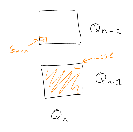
Claim: $| \partial B_{i} (A) | \leq | \partial A |$ .

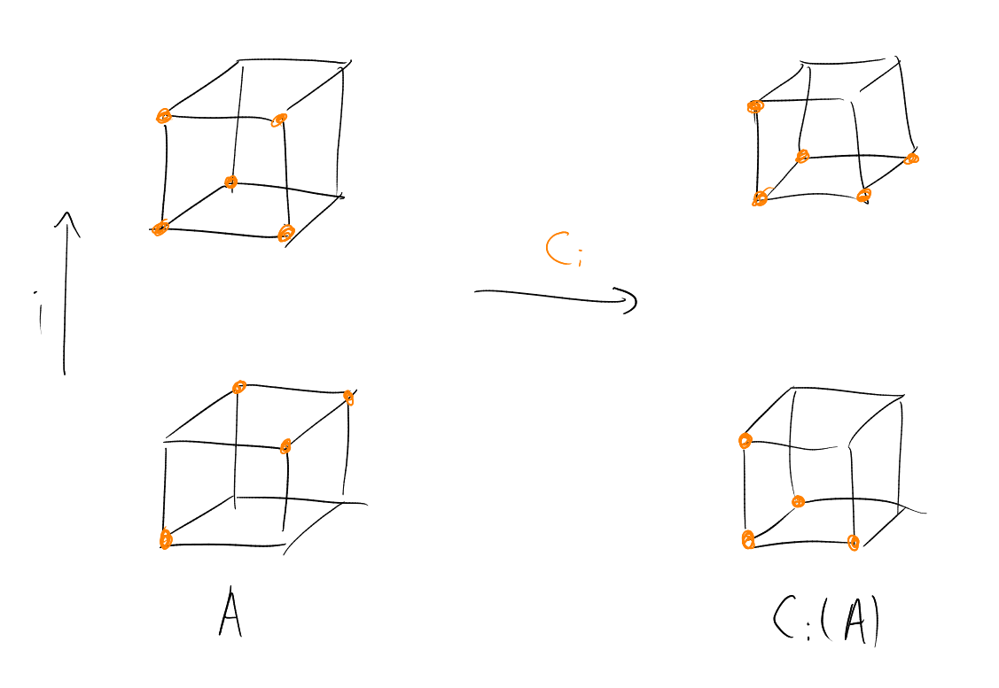
Proof of claim: write $B$ for $B_{i} (A)$ . .image Have

|∂A| = |∂(A )| +|∂(A )|+ |A ΔA |
◟-◝−◜-◞ ◟--◝+◜-◞ ◟-+◝◜-−◞
downstairs upstairs across

Also

| \partial B | = | \partial (B_{-}) | + | \partial (B_{+}) | + | B_{+} Δ B_{-} | .

Now, $| \partial (B_{-}) | \leq | \partial (A_{-}) |$ and $| \partial (B_{+}) | \leq | \partial (A_{+}) |$ (induction hypothesis). Also, the sets $B_{+}$ and $B_{-}$ are nested (one is contained inside the other), as each is an initial segment of binary on $P (X - i)$ .

Whence we certainly have $| B_{+} Δ B_{-} | \leq | A_{+} Δ A_{-} |$ . So $| \partial B | \leq | \partial A |$ .

Define a sequence $A_{0}, A_{1}, \dots \subset Q_{n}$ as follows: set $A_{0} = A$ . Having defined $A_{0}, \dots, A_{k}$ , if $A_{k}$ is $i$ -binary compressed for all $n$ then stop the sequence with $A_{k}$ . If not, choose $i$ with $B_{i} (A) \neq A$ and put $A_{k + 1} = B_{i} (A_{k})$ . Must terminate, as the function $k \mapsto \sum_{x \in A_{k}} (position of x in binary)$ is strictly decreasing.

The final family $B = A_{k}$ satisfies $| B | = | A |$ , $| \partial B | \leq | \partial A |$ , and $B$ is $i$ -binary compressed for all $i$ .

Note that $B$ need not be an initial segment of binary, for example ${\emptyset, 1, 2, 3} \subset Q_{3}$ .

However:

Lemma 9. Assuming that:

$B \subset Q_{n}$ is $i$ -binary compressed for all $i$
$B$ not an initial segment of binary

Then

B = P (n - 1) - {1, 2, 3, \dots, n - 1} \cup {n}

(“downstairs minus the last point, plus the first upstairs point”).

(Then done, as clearly $| \partial B | \geq | \partial C |$ , since $C = P (n - 1)$ ).

Proof. As $B$ not an initial segment, there exists $x < y$ with $x \notin B$ , $y \in B$ . Then for all $i$ : cannot have $i \in x, y$ , and cannot have $i \notin x, y$ (as $B$ is $i$ -binary compressed).

Thus for each $y \in B$ , there exists at most 1 earlier $x \notin B$ (namely $x = y^{c}$ ). Also for each $x \notin B$ there is at most one later $y \in B$ (namely $y = x^{c}$ ).

Then $x$ and $y$ adjacent (since $y$ is the unique element in $B$ after $x$ , and $x$ is the unique element not in $B$ before $y$ ).

So $B = {z : z \leq y} - {x}$ , where $x$ is the predecessor of $y$ and $y = x^{c}$ .

So must have $y = {n}$ . □

This concludes the proof of Theorem 8. □

Remark. Vital in the proof of Theorem 8, and of Theorem 1, that the extremal sets (in dimension $n - 1$ ) were nested.

The isoperimetric number of a graph $G$ is

i (G) = \min {\frac{| \partial A |}{| A |} : A \subset G, \frac{| A |}{| G |} \leq \frac{1}{2}} .

$\frac{| \partial A |}{| A |}$ is the “average out-degree of $| A |$ ”.

Corollary 10. $i (Q_{n}) = 1$ .

Proof. Taking $A = P (n - 1)$ , we show $i (Q_{n}) \leq 1$ (as $\frac{| \partial A |}{| A |} = \frac{2^{n - 1}}{2^{n}} = \frac{1}{2}$ ).

To show $i (Q_{n}) \geq \frac{1}{2}$ , just need to show that if $C$ is an initial segment of binary with $| C | \leq 2^{n - 1}$ then $| \partial C | \geq | C |$ .

But $C \subset P (n - 1)$ , so certainly $| \partial C | \geq | C |$ . □

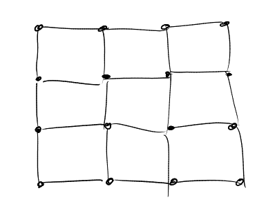
2.3 Inequalities in the grid

For any $k = 2, 3, \dots$ , the grid is the graph on ${[k]}^{n}$ in which $x$ is joined to $y$ if for some $i$ we have $x_{j} = y_{j}$ for all $j \neq i$ and $| x_{i} - y_{i} | = 1$ .

“distance is $l_{1}$ -distance”.

Example. ${[4]}^{2}$

Note that for $k = 2$ this is exactly $Q_{n}$ .

Do we have analogues of Theorem 1 and Theorem 8 for the grid?

Starting with vertex-isoperimetric: which sets $A \subset {[k]}^{n}$ (of given size) minimise $| N (A) |$ ?

Example. In ${[k]}^{2}$ :

For $A$ : $| b (A) | \sim r \sim \sqrt{2 | A |}$ .

For $B$ : $| b (B) | = 2 r = 2 \sqrt{| B |}$ .

This suggests we “go up in levels” according to $| x | = \sum_{i = 1}^{n} | x_{i} |$ – e.g. we’d take ${x \in {[k]}^{n} : | x | \leq r}$ .

What if $| {x \in {[k]}^{n} : | x | \leq r} | < | A | < | {x \in {[k]}^{n} : | x | \leq r + 1}$ ?

Guess: take $A = {x \in {[k]}^{n} : | x | \leq r}$ plus some points with $| x | = r + 1$ , but which points?

Example. In ${[k]}^{3}$ :

so “keep $x_{1}$ large”.

This suggests in the simplicial order on ${[k]}^{n}$ , we set $x < y$ if either $| x | < | y |$ or $| x | = | y |$ and $x_{i} > y_{i}$ , where $i = \min, c b j : x_{j} \neq y_{j}}$ .

Note. Agrees with the previous definition of simplicial ordering when $k = 2$ .

Example. On ${[3]}^{2}$ : $(1, 1)$ , $(2, 1)$ , $(1, 2)$ , $(1, 1)$ , $(2, 2)$ , $(1, 3)$ , $(3, 2)$ , $(2, 3)$ , $(3, 3)$ .

On ${[4]}^{3}$ : $(1, 1, 1)$ , $(2, 1, 1)$ , $(1, 2, 1)$ , $(1, 1, 2)$ , $(3, 1, 1)$ , $(2, 2, 1)$ , $(2, 1, 2)$ , $(1, 3, 1)$ , $(1, 2, 2)$ , $(1, 1, 3)$ , $(4, 1, 1)$ , $(3, 2, 1)$ , …

r $A \subset {[k]}^{n}$ ( $n \geq 2$ ), and $1 \leq i \leq n$ , the $i$ -sections of $A$ are the sets $A_{1}, \dots, A_{k}$ (or $A_{1}^{(i)}, \dots, A_{k}^{(i)}$ ) as a subset of ${[k]}^{n - 1}$ defined by:

A_{t} = {x \in {[k]}^{n - 1} : (x_{1}, x_{2}, \dots, x_{i - 1}, t, x_{i}, x_{i + 1}, \dots, x_{n - 1}) \in A},

for each $1 \leq t \leq k$ .

The $i$ -compression of $A$ is $C_{i} (A) \subset {[k]}^{n}$ is defined by giving its $i$ -sections:

C_{i} {(A)}_{t} = initial segment of {[k]}^{n - 1} of size | A_{t} |, for each 1 \leq t \leq k .

Thus $| C_{i} (A) | = | A |$ .

Say $A$ is $i$ -compressed if $C_{i} (A) = A$ .

Theorem 11 (Vertex-isoperimetric inequality in the grid). Assuming that:

$A \subset {[k]}^{n}$
$C$ is the initial segment of simplicial order on ${[k]}^{n}$ with $| C | = | A |$

Then

| N (C) | \leq | N (A) |

. In particular, if

| A | \geq | {x : | x | \leq r} |

then

| N (A) | \geq | {x : | x | \leq r + 1} |

Proof. Induction on $n$ . For $n = 1$ it is trivial: if $A \subset {[k]}^{1} \neq \emptyset, {[k]}^{1}$ , then $| N (A) | \geq | A | + 1 = | N (C) |$ .

Given $n > 1$ and $A \subset {[k]}^{n}$ : fix $1 \leq i \leq n$ .

Claim: $| N (C_{i} (A) | \leq | N (A) |$ .

Proof of claim: write $B$ for $C_{i} (A)$ . For any $1 \leq t \leq k$ , we have

N {(A)}_{t} = \underset{from x_{i} = t}{\underset{⏟}{N (A_{t})}} \cup \underset{from x_{i} = t - 1}{\underset{⏟}{A_{t - 1}}} \cup \underset{from x_{i} = t + 1}{\underset{⏟}{A_{t + 1}}} .

(where $A_{0}, A_{k + 1} = \emptyset$ ).

Also,

N {(B)}_{t} = N (B_{t}) \cup B_{t - 1} \cup B_{t + 1} .

Now, $| B_{t - 1} | = | A_{t - 1} |$ and $| B_{t + 1} | = | A_{t + 1} |$ , and $| N (B_{t}) | \leq | N (A_{t}) |$ (induction hypothesis). But the sets $B_{t - 1}$ , $B_{t + 1}$ , $N (B_{t})$ are nested (as each is an initial segment of simplicial order on ${[k]}^{n - 1}$ ).

Hence $| N {(B)}_{t} | \leq | N {(A)}_{t} |$ for each $t$ . Thus $| N (B) | \leq | N (A) |$ .

Among all $B \subset {[k]}^{n}$ with $| B | = | A |$ and $| N (B) | \leq | N (A) |$ , pick one that minimises the quantity $\sum_{x \in B} position of x in simplicial order$ .

Then $B$ is $i$ -compressed for all $i$ . Note however, that this time we will make use of this minimality property of $B$ for more than just deducing that $B$ is $i$ -compressed for all $i$ .

Case 1: $n = 2$ . What we know is precisely that $B$ is a down-set ( $A \subset {[k]}^{n}$ is a down-set if $x \in A$ , $y_{i} \leq x_{i} \forall i ⟹ y \in A$ )

Let $r = \min {| x | : x \notin B}$ and $s = \max {| x | : x \notin B}$ . May assume $r \leq s$ , since $r = s + 1$ implies $B = {x : | x | \leq r - 1}$ would imply $B = C$ .

If $r = s$ : then ${x : | x | \leq r - 1} \subset B \subset {x : | x | \leq r}$ . So clearly $| N (B) | \geq | N (C) |$ .

If $r < s$ : cannot have ${x : | x | = s} \subset B$ , because then also ${x : | x | = r} \subset B$ (as $B$ is a down-set).

So there exists $y, y^{'}$ with $| y | = | y^{'} | = s$ , $y \in B$ , $y^{'} \notin B$ and $y^{'} = y \pm (e_{1} - e_{2})$ ( $e_{1} = (1, 0)$ , $e_{2} = (0, 1)$ ).

Similarly, cannot have ${x : | x | = r} \cap B = \emptyset$ , because then ${x : | x | = s} \cap B = \emptyset$ (as $B$ is a down-set). So there exists $x, x^{'}$ with $| x | = | x^{'} | = r$ , $x \notin B$ , $x^{'} \in B$ and $x^{'} = x \pm (e_{1} - e_{n})$ . Now let $B^{'} = B \cup {x} - {y}$ . From $B$ we lost $\geq 1$ point in the neighbourhood (namely $z$ in the picture), and gained $\leq 1$ point (the only point that we can possibly gain is $w$ ), so $| N (B^{'}) | \leq | N (B) |$ . This contradicts minimality of $B$ . This finishes the two dimensional case.

Case 2: $n \geq 3$ . For any $1 \leq i \leq n - 1$ and any $x \in B$ with $x_{n} > 1$ , $x_{i} < k$ . Have $x - r_{n} + e_{i} \in B$ (as $B$ is $j$ -compressed for any $j$ , so apply with some $j \neq i, n$ ). So, considering the $n$ -sections of $B$ , we have $N (B_{t}) \subset B_{t - 1}$ for all $t = 2, \dots, k$ .

Recall that $N {(B)}_{t} = N (B_{t}) \cup B_{t + 1} \cup B_{t - 1}$ . So in fact $N {(B)}_{t} = B_{t - 1}$ for all $t \geq 2$ . Thus

| N (B) | = \underset{level k}{\underset{⏟}{| B_{k - 1} |}} + \underset{level k - 1}{\underset{⏟}{| B_{k - 2} |}} + \dots + \underset{level 2}{\underset{⏟}{| B_{1} |}} + \underset{level 1}{\underset{⏟}{| N (B_{1}) |}} = | B | - | B_{k} | + | N (B_{1}) | .

Similarly,

| N (C) | = | C | - | C_{k} | + | N (C_{1}) | .

So to show $| N (C) | \leq | N (B) |$ , enough to show that $| B_{k} | \leq | C_{k} |$ and $| B_{1} | \geq | C_{1} |$ .

$| B_{k} | \leq | C_{k} |$ : define a set $D \subset {[k]}^{n}$ as follows: put $D_{k} = B_{k}$ , and for $t = k - 1, k - 2, \dots, 1$ set $D_{t} = N (D_{t - 1})$ . Then $D \subset B$ , so $| D | \leq | B |$ . Also, $D$ is an initial segment of simplicial order. So in fact $D \subset C$ , whence $| B_{k} | = | D_{k} | \leq | C_{k} |$ .

$| B_{1} | \geq | C_{1} |$ : define a set $E \subset {[k]}^{n}$ as follows: put $E_{1} = B_{1}$ and for $t = 2, 3, \dots, k$ set $E_{t} = {x \in {[k]}^{n - 1} : N ({x}) \subset E_{t - 1}}$ ( $E_{t}$ is the biggest it could be given $N (E_{t}) \subset E_{t}$ ). Then $E \supset B$ , so $| E | \geq | B |$ . Also, $E$ is an initial segment of simplicial order. So $E \supset C$ , whence $| B_{1} | = | E_{1} | \geq | C_{1} |$ . □

Corollary 12. Let $A \subset {[k]}^{n}$ with $| A | \geq | {x : | x | \leq n} |$ . Then $| A_{(t)} | \geq | {x : | x | \leq r + t} |$ for all $t$ .

Remark. Can check from Corollary 12 that, for $k$ fixed, the sequence ${({[k]}^{n})}_{n = 1}^{\infty}$ is a Lévy family.

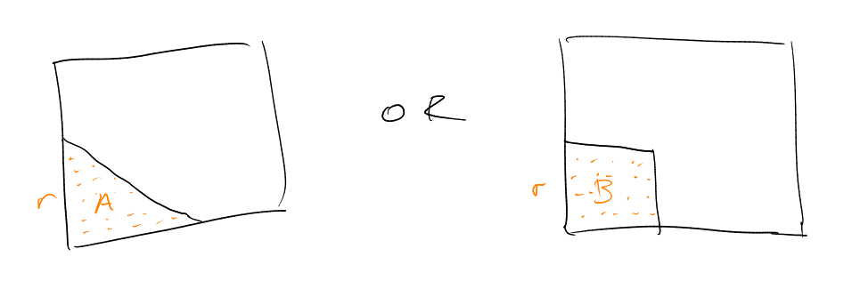
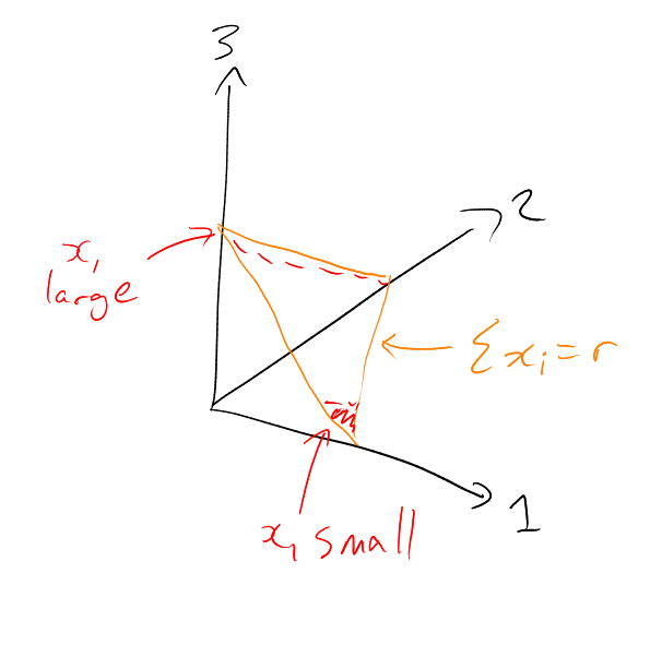
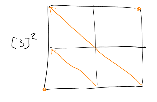
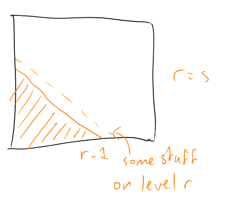
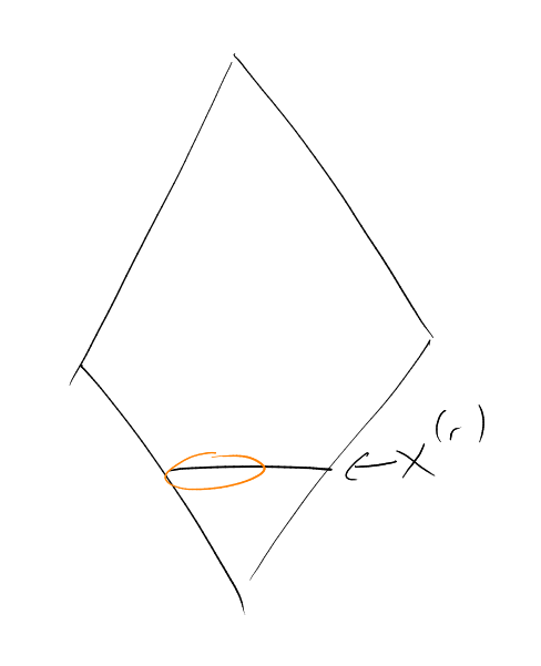
2.4 The edge-isoperimetric inequality in the grid

Which set $A \subset {[k]}^{n}$ (of given size) should we take to minimise $| \partial A |$ ?

Example. In ${[k]}^{n}$ :

Suggests squares are best.

However...

So we have “phase transitions” at $| A | = \frac{k^{2}}{4}$ and $\frac{3 k^{2}}{4}$ – extremal sets are not nested. This seems to rule out all our compression methods.

And in ${[k]}^{3}$ ?

\begin{array}{l} {[a]}^{3} (cube) & ⇝ {[a]}^{2} \times [k] (square column) \\ ⇝ [a] \times {[k]}^{2} (half space) \\ ⇝ complement of square column \\ ⇝ complement of cube \end{array}

So in ${[k]}^{n}$ , up to $| A | = \frac{k^{n}}{2}$ , we get $n - 1$ of these phase transitions!

Note that if $A = [a] \times {[k]}^{n - d}$ . Then $| \partial A | = d a^{d - 1} k^{n - d} = d | A |^{1 - \frac{1}{d}} k^{\frac{n}{d} - 1}$ .

Theorem 13. Assuming that:

$A \subset {[k]}^{n}$
$| A | \leq \frac{k^{n}}{2}$

Then

| \partial A | \geq \min {d | A |^{1 - \frac{1}{d}} k^{\frac{n}{d} - 1} : 1 \leq d \leq n} .

“Some set of the form ${[a]}^{d} \times {[k]}^{n - d}$ is best.”

Called the “edge-isoperimetric inequality in the grid”.

The following discussion is non-examinable (until told otherwise).

Proof (sketch). Induction on $n$ . $n = 1$ is trivial.

Given $A \subset {[k]}^{n}$ with $| A | \leq \frac{k^{n}}{2}$ , where $n > 1$ :

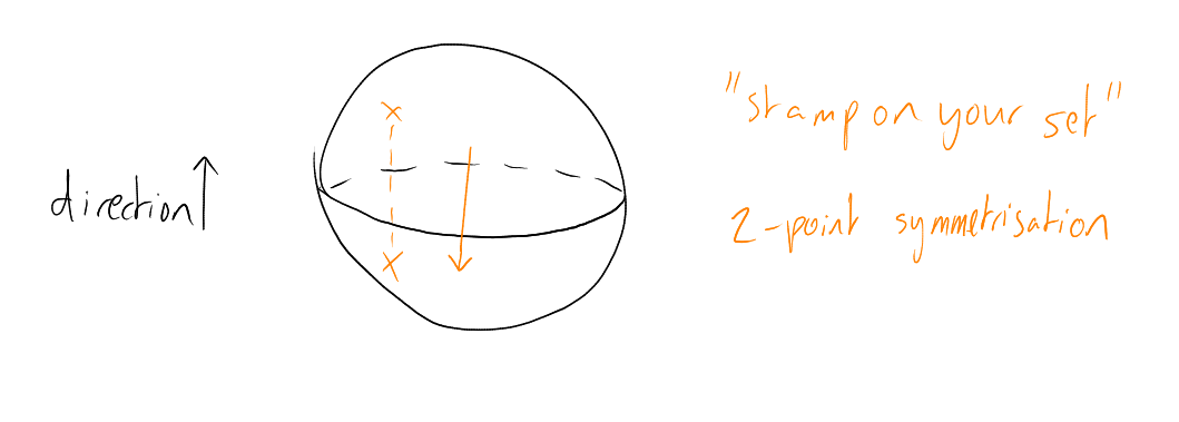
Wlog $A$ is a down-set (just down-compress, i.e. stamp on your set in direction $i$ for each $i$ ). For any $1 \leq i \leq n$ , define $C_{i} (A) \subset {[k]}^{n}$ by giving its $i$ -sections:

C_{i} {(A)}_{t} = extremal set of size | A_{t} | in {[k]}^{n - 1},

which will be a set of the form ${[a]}^{d} \times {[k]}^{n - 1 - d}$ , or a complement. Write $B = C_{i} (A)$ . Do we have $| \partial B | \leq | \partial A |$ ?

Now, $A$ is a down-set, so

| \partial A | = \underset{horizontal edges}{\underset{⏟}{| \partial A_{1} | + \dots + | \partial A_{k} |}} + \underset{vertical edges}{\underset{⏟}{| A_{1} | - | A_{k} |}}

and

| \partial B | = | \partial B_{1} | + \dots + | \partial B_{k} | + ?

The $?$ is because $B$ not a down-set, as extremal sets in dimension $n - 1$ are not nested.

Indeed, can have $| \partial B | > | \partial A |$ :

Idea: try to introduce a “fake” boundary $\partial^{'}$ : want $\partial^{'} A \leq \partial A$ , with $\partial^{'} = \partial$ on extremal sets, such that $C_{i}$ does decrease $\partial^{'}$ (then done).

Try $\partial^{'} A = \sum_{t} | \partial A_{t} | + | A_{1} | - | A_{k} |$ . Then $\partial^{'} A \leq | \partial A |$ for all $A$ , equality for extremal sets (as equality for any down-set) and $\partial^{'} C_{i} (A) \leq \partial^{'} A$ . But: fails for $C_{j} (A)$ for all $j \neq i$ .

Could try to fix this by defining $\partial^{″} A = \sum_{i} (| A_{1}^{(i)} | - | A_{k}^{(i)} |)$ . Also fails – for example if $A$ is the “outer shell” of ${[k]}^{n}$ then $\partial^{″} A = 0$ .

So far, have

\begin{array}{l} | \partial A | & \geq \partial^{'} A \\ \geq \partial^{'} B \\ = \sum_{t} | \partial B_{t} | + | B_{1} | - | B_{k} | \\ = \sum_{t} f (| B_{t} |) + | B_{1} | - | B_{k} | \end{array}

where $f$ is the extremal function in ${[k]}^{n - 1}$ .

Now, $f$ is the pointwise minimum of some functions of the form $c x^{1 - \frac{1}{d}}$ and $c {(k^{n - 1} - x)}^{1 - \frac{1}{d}}$ – each of which is a concave function. Hence $f$ itself is a concave function.

Consider varying $| B_{2} |, \dots, | B_{k - 1} |$ , keeping $| B_{2} | + \dots + | B_{k - 1} |$ constant and keeping $| B_{1} | \geq | B_{2} | \geq \dots \geq | B_{k - 1} | \geq | B_{k} |$ .

We obtain $\partial^{'} B \geq \partial^{'} C$ , where for some $λ$ ,

C_{t} = {\begin{matrix} B_{1} & \forall 1 \leq t \leq λ \\ B_{k} & \forall λ + 1 \leq t \leq k \end{matrix}

So:

\begin{array}{l} | \partial A | & = \partial^{'} A \\ \geq \partial^{'} B \\ \geq \partial^{'} C \\ = λ f (| B_{1} |) + (k - λ) f (| B_{k} |) + | B_{1} | - | B_{k} | \end{array}

but $C$ is still not a down-set.

Now vary, $| B_{1} |$ , keeping $λ | B_{1} | + (k - λ) | B_{k} |$ fixed ( $λ$ fixed) and $| B_{1} | \geq | B_{k} |$ .

This is a concave function of $| B_{1} |$ – as concave + concave + linear. Hence “make $| B_{1} |$ as small or large as possible”.

i.e. $\partial^{'} C \geq \partial^{'} D$ , where one of the following holds:

$D_{t} = D_{1}$ for all $t$
$D_{t} = D_{1}$ for all $t \leq λ$ , $D_{t} = \emptyset$ for all $t > λ$
$D_{t} = {[k]}^{n - 1}$ for all $t \leq λ$ , $D_{t} = D_{k}$ for all $t > λ$ .

But (miraculously), this $D$ is a down-set!

Hence

| \partial A | = \partial^{'} A \geq \partial^{'} B \geq \partial^{'} C \geq \partial^{'} D = | \partial D | .

So our “compression in direction $i$ ” is: $A \mapsto D$ .

Now finish as before. □

Remark. To make this precise, work instead in ${[0, 1]}^{n}$ (and then take a discrete approximation at the end).

End of non-examinable discussion.

Remark. Very few isoperimetric inequalities are known (even approximately).

For example, “isoperimetric in a layer” – in the graph $X^{(r)}$ , with $x, y$ joined if $| x \cap y | = r - 1$ (i.e. $d (x, y) = 2$ in $Q_{n}$ ).

This is open. Nicest special case is $r = \frac{n}{2}$ , where it is conjectured that balls are best – i.e. sets of the form ${x \in {[r]}^{(r)} : | x \cap [r] | \geq t}$ .

3 Intersecting Families

3.1 $t$ -intersecting families

$A \subset P (X)$ is called $t$ -intersecting if $| x \cap y | \geq t$ for all $x, y \in A$ .

How large can a $t$ -intersecting family be?

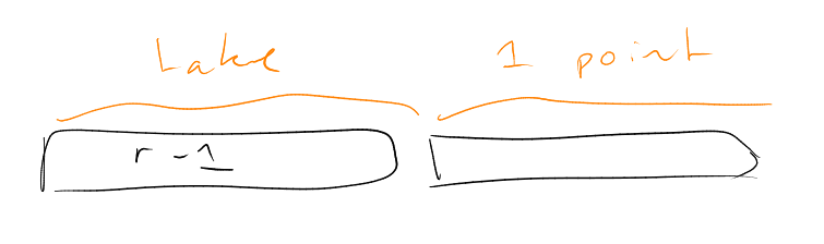
Example. $t = 2$ . Could take ${x : 1, 2 \in x}$ – has size $\frac{1}{4} 2^{n}$ . Or ${x : | x | \geq \frac{n}{2} + 1}$ – has size $\sim \frac{1}{2} 2^{n}$ .

Theorem 1 (Katona’s $t$ -intersecting Theorem). Assuming that:

$A \subset P (X)$ is $t$ -intersecting
$n + t$ even (to make the proof simpler – same proof works for odd)

Then

| A | \leq | X^{(\geq \frac{n + t}{2})} |

Proof. For any $x, y \in A$ : have $| x \cap y | \geq t$ , so $d (x, y^{c}) \geq t$ . So, writing $\bar{A}$ for ${y^{c} : y \in A}$ , have $d (A, \bar{A}) \geq t$ – i.e. $A_{(t - 1)}$ disjoint from $\bar{A}$ . Suppose that $| A | > | X^{(\geq \frac{n + t}{2})} |$ .

Then, by Harper’s Theorem, we have

| A_{(t - 1)} | \geq | X^{(\geq \frac{n + t}{2} - (t - 1))} | = | X^{(\geq \frac{n - t}{2} + 1)} | .

But $A_{(t - 1)}$ disjoint from $\bar{A}$ , which has size $> | X^{(\leq \frac{n - t}{2})} |$ contradicting $| A_{(t - 1)} | + | \bar{A} | \leq 2^{n}$ . □

What about $t$ -intersecting $A \subset X^{(r)}$ ?

Might guess: best is $A_{0} = {x \in X^{(r)} : [t] \subset x}$ .

Could also try $A_{α} = {x \in X^{(r)} : | x \cap [t + 2 α] | \geq t + α}$ , for $α = 1, 2, \dots, r - t$ .

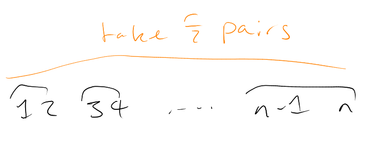
Example. For $2$ -intersecting in:

${[7]}^{(4)}$ : $| A_{0} | = (\binom{5}{2}) = 10$ , $| A_{1} | = 1 + (\binom{4}{3}) (\binom{3}{1}) = 13$ , $| A_{2} | = (\binom{6}{4}) = 15$ .
${[8]}^{(4)}$ : $| A_{0} | = (\binom{6}{2}) = 15$ , $| A_{1} | = 1 + (\binom{4}{3}) (\binom{4}{1}) = 17$ , $| A_{2} | = (\binom{6}{4}) = 15$ .
${[9]}^{(4)}$ : $| A_{0} | = (\binom{7}{2}) = 21$ , $| A_{1} | = 1 + (\binom{4}{3}) (\binom{5}{1}) = 21$ , $| A_{2} | = (\binom{6}{4}) = 15$ .

Note that $| A_{0} |$ grows quadratically, $| A_{1} |$ linearly, and $| A_{2} |$ constant – so $| A_{0} |$ largest of these for $n$ large.

Theorem 2. Assuming that:

$A \subset X^{(r)}$ is $t$ -intersecting

Then for

n

sufficiently large, we have

| A | \leq | A_{0} | = (\binom{n - t}{r - t})

Remark.

(1) Bound we get on $n$ would be ${(16 r)}^{r}$ (crude) or $2 t r^{3}$ (careful).
(2) Often called the “second Erdős-Ko-Rado Theorem”.

Idea of proof: “ $A_{0}$ has $r - t$ degrees of freedom”.

Proof. Extending $A$ to a maximal $t$ -intersecting family, we must have some $x, y \in A$ with $| x \cap y | = t$ (if not, then by maximality have that $\forall x \in A$ , $\forall i \in x$ , $\forall j \notin x$ , have $x \cup j - i \in A$ – whence $A = X^{(r)}$ , contradiction).

May assume that there exists $z \in A$ with $x \cap y ⁄ \subset z$ – otherwise all $z \in A$ have $x \cap y \subset z$ . Whence $| A | \leq (\binom{n - t}{r - t}) = | A_{0} |$ .

So each $w \in A$ must meet $x \cup y \cup z$ in $\geq t + 1$ points. Thus

| A | \leq \underset{w on x \cup y \cup z}{\underset{⏟}{2^{3 r}}} (\underset{w off x \cup y \cup z}{\underset{⏟}{(\binom{n}{r - t - 1}) + (\binom{n}{r - t - 2}) + \dots + (\binom{n}{0})}}) .

Note that the right hand side is a polynomial of degree $r - t - 1$ – so eventually beaten by $| A_{0} |$ . □

3.2 Modular Intersections

For intersecting families, we ban $| x \cap y | = 0$ .

What if we banned $| x \cap y | \equiv 0 (m o d something)$ ?

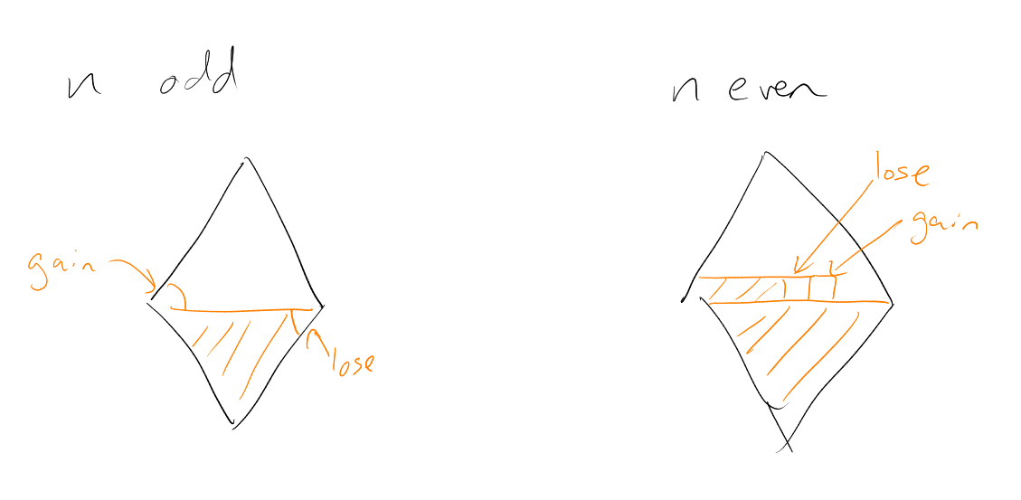
Example. Want $A \subset X^{(r)}$ with $| x \cap y |$ odd for all distinct $x, y \in A$ ?

Try $r$ odd: can achieve $| A | = (\binom{⌊ \frac{n - 1}{2} ⌋}{\frac{r - 1}{2}})$ , by picture.

What if, still for $r$ odd, had $| x \cap y |$ even for all distinct $x, y \in A$ ? Can achieve $n - r + 1$ , by picture.

This is only linear in $n$ . Can we improve this?

Similarly if $r$ even: For $| x \cap y |$ even for all $x, y \in A$ , can achieve $| A | = (\binom{⌊ \frac{n}{2} ⌋}{\frac{r}{2}})$ – picture

But for $| x \cap y |$ odd for all $x, y \in A$ (distinct): can achieve $n - r + 1$ (as above). Can we improve this?

Seems to be that banning $| x \cap y | = r (m o d 2)$ forces the family to be very small (polynomial in $n$ , in fact a linear polynomial).

Remarkably, cannot beat linear.

Proposition 3. Assuming that:

$r$ is odd
$A \subset X^{(r)}$ such that $| x \cap y |$ for each distinct $x, y \in A$

Then

| A | \leq n

Idea: Find $| A |$ linearly independent vectors in a vector space of dimension $n$ , namely $Q_{n}$ .

Proof. View $P (X)$ as $ℤ_{2}^{n}$ , the $n$ -dimensional space over $ℤ_{2}$ (the field of order $2$ ). By identifying $x$ with $\bar{x}$ , its characteristic sequence (e.g. $1011000 \dots$ for ${1, 3, 4}$ ).

We have $(\bar{x}, \bar{x}) \neq 0$ for each $x$ , as $r$ is odd ( $(∙, ∙)$ is the usual dot-product).

Also, $(\bar{x}, \bar{y}) = 0$ for distinct $x, y \in A$ (as $| x \cap y |$ even).

Hence the $\bar{x}$ , $x \in A$ are linearly independent (if $\sum λ_{i} \bar{x_{i}} = 0$ , dot with $\bar{x_{j}}$ to get $λ_{j} = 0$ ). □

Remark. Hence also if $A \subset X^{(r)}$ , $r$ even, with $| x \cap y |$ odd for all distinct $x, y \in A$ , then $| A | \leq n + 1$ – just add $n + 1$ to each $x \in A$ and apply Proposition 3 with $X = [n + 1]$ .

Does this modulo $2$ behaviour generalise?

Now show: $s$ allowed values for $| x \cap y |$ modulo $p$ implies $| A | \leq$ polynomial of degree $s$ .

Theorem 4 (Frankl-Wilson Theorem). Assuming that:

$p$ is prime
$λ_{1}, \dots, λ_{s}$ ( $s \leq r$ )
$λ_{i} ⁄ \equiv r (m o d p)$ for each $i$
$A \subset X^{(r)}$ such that for all distinct $x, y \in A$ have $| x \cap y | \equiv λ_{i} (m o d p)$ for some $i$

Then

| A | \leq (\binom{n}{s})

Remark.

(1) This bound is a polynomial in $S$ (as $r$ vares)!
(2) Bound is essentially best possible: can achieve $| A | = (\binom{n}{n - r + s}) \sim (\binom{n}{s})$ (see picture).
(3) Do need no $λ_{i} \equiv r (m o d p)$ . Indeed, if $n = a + λ p$ ( $0 \leq a \leq p - 1$ ) then can have $A \subset^{(a + k p)}$ with $| A | = (\binom{λ}{k})$ (not a polynomial in $n$ , as we can choose any $k$ ) and all $| x \cap y | \equiv a (m o d p)$ .

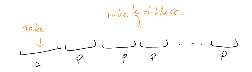
Idea: Try to find $| A |$ linearly independent points in a vector space of dimension $(\binom{n}{s})$ , by somehow “applying the polynomial $(t - λ_{1}) \dots (t - λ_{s})$ to $| x \cap y |$ ”.

Proof. For each $i \leq j$ , let $M (i, j)$ be the $(\binom{n}{i}) \times (\binom{n}{j})$ matrix, with rows indexed by $X^{(i)}$ , columns indexed by $X^{(j)}$ , with

M {(i, j)}_{x y} = {\begin{matrix} 1 & if x \subset y \\ 0 & otherwise \end{matrix}

for each $x \in X^{(i)}$ , $y \in X^{(j)}$ .

Let $V$ be the vector space (over $ℝ$ ) spanned by the rows of $M (s, r)$ . So $\dim V \leq (\binom{n}{s})$ .

For $i \leq s$ , consider $M (i, s) M (s, r)$ (note each row belongs to $V$ , as we premultiplied $M (s, r)$ by a matrix). For $x \in X^{(i)}$ , $y \in X^{(r)}$ :

\begin{array}{l} {(M (i, s) M (s, r))}_{x y} & = # of s -sets z with x \subset z and z \subset y \\ = {\begin{matrix} 0 & if x ⁄ \subset y \\ (\binom{r - i}{s - i}) & if x \subset y \end{matrix} \end{array}

M (i, s) M (s, r) = (\binom{r - i}{s - i}) M (i, r)

so all rows of $M (i, r)$ belong to $V$ .

Let $M (i) = M {(i, r)}^{⊤} M (i, r)$ (note each row is in $V$ ).

For $x, y \in X^{(r)}$ , have

\begin{array}{l} M {(i)}_{x y} & = # i -sets z with z \subset x, z \subset y \\ = (\binom{| x \cap y |}{i}) \end{array}

Write the integer polynomial $(t - λ_{1}) \dots (t - λ_{s})$ as $\sum_{i = 0}^{s} a_{i} (\binom{t}{i})$ , with $a_{i} \in ℤ$ – possible because $t (t - 1) \dots (t - i + 1) = i! (\binom{t}{i})$ .

Let $M = \sum_{i = 0}^{s} a_{i} M^{(i)}$ (each row is in $V$ ).

Then for all $x, y \in X^{(r)}$ :

M_{x y} = \sum_{i} a_{i} (\binom{| x \cap y |}{i}) = (| x \cap y | - λ_{i}) \dots (| x \cap y | - λ_{s}) .

So the submatrix of $M$ spanned by the rows and columns corresponding to the elements of $A$ is

(\begin{matrix} ⁄ \equiv 0 & 0 & \dots & 0 \\ 0 & ⁄ \equiv 0 & \dots & 0 \\ ⋮ & ⋮ & ⋱ & ⋮ \\ 0 & 0 & \dots & ⁄ \equiv 0 \end{matrix}) .

Hence the rows of $M$ corresponding to $A$ are linearly independent over $ℤ_{p}$ , so also over $ℤ$ , so also over $ℚ$ , so also over $ℝ$ .

So $| A | \leq \dim V \leq (\binom{n}{s})$ . □

Remark. Do need $p$ prime. Grolmusz constructed, for each $n$ , a value of $r \equiv 0 (m o d 6)$ and a family $A \subset {[n]}^{(r)}$ such that for all distinct $x, y \in A$ we have $| x \cap y | ⁄ \equiv 0 (m o d 6)$ with $| A | > n^{c \log n ∕ \log \log n}$ . This is not a polynomial in $n$ .

Corollary 5. Let $A \subset {[n]}^{(r)}$ with $| x \cap y | ⁄ \equiv r (m o d p)$ , for each distinct $x, y \in A$ , where $p < r$ is prime.

Proof. We are allowed $p - 1$ values of $| x \cap y | (m o d p)$ , so done by Frankl-Wilson Theorem. □

Two $\frac{n}{2}$ -sets in $[n]$ typically meet in about $\frac{n}{4}$ points – but $| x \cap y |$ exactly equaling $\frac{n}{4}$ is very unlikely. But remarkably:

Corollary 6. Let $p$ be prime, and let $A \subset {[4 p]}^{(2 p)}$ have $| x \cap y | \neq p$ for all distinct $x, y \in A$ (“this is not much of a constraint”). Then $| A | \leq 2 (\binom{4 p}{p - 1})$ .

Note. $(\binom{4 p}{p - 1})$ is a tiny (exponentially small) proportion of $(\binom{4 p}{2 p})$ . Indeed, $(\binom{n}{n ∕ 2}) \sim c \cdot \frac{2^{n}}{\sqrt{n}}$ (for some $c$ ) whereas $(\binom{n}{n ∕ 4}) \leq 2 e^{- n ∕ 32} 2^{n}$ .

Proof. Halving $| A |$ if necessary, may assume that no $x, x^{c} \in A$ (any $x \in {[4 p]}^{(2 p)}$ ).

Then $x, y \in A$ distinct implies $| x \cap y | \neq 0, p$ , so $| x \cap y | ⁄ \equiv 0 (m o d p)$ .

So $| A | \leq (\binom{4 p}{p - 1})$ by Corollary 5. □

3.3 Borsuk’s Conjecture

Let $S$ be a bounded subset of $ℝ^{n}$ .

How few pieces can we break $S$ into such that each piece has smaller diameter than that of $S$ ?

The example of a regular simplex in $ℝ^{n}$ ( $n + 1$ points, all at distance $1$ ) shows that we may need $n + 1$ pieces.

Conjecture (Borsuk’s conjecture (1920s)). $n + 1$ pieces always sufficient.

Known for $n = 1, 2, 3$ . Also known for $S$ a smooth convex body in $ℝ^{n}$ or a symmetric convex body in $ℝ^{n}$ (convex means $x \in S$ implies $- x \in S$ ).

However, Borsuk is massively false:

Theorem 7 (Kahn, Kalai 1995). Assuming that:

$n \in ℕ$

Then there exists bounded

S \subset ℝ^{n}

such that to break

S

into pieces of smaller diameter we need

\geq C^{\sqrt{n}}

, for some constant

c > 1

(not depending on

n

Note.

(1) Our proof will show Borsuk’s conjecture (1920s) is false for $n \geq 2000$ .
(2) We’ll prove it for $n$ of the form $(\binom{4 p}{2})$ , where $p$ is prime. Then done for all $n$ (with a different $c$ , e.g. because there exists a prime $p$ with $\frac{n}{2} \leq p \leq n$ ).

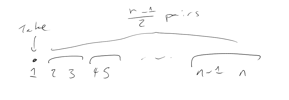
Proof. We’ll find $S \subset Q_{n} \subset ℝ^{n}$ – in fact $S \subset {[n]}^{(r)}$ for some $r$ . We have already had two genuine ideas from this sentence: first that we think about having $S \subset Q_{n}$ , and second that we go for $S \subset {[n]}^{(r)}$ .

Have $S \subset {[n]}^{(r)}$ , so $\forall x, y \in S$ :

∥ x - y ∥^{2} = # coordinates where x and y differ = 2 (r - | x \cap y |) .

So seek $S$ with diameter $\min | x \cap y | = k$ , but every subset of $S$ with $\min | x \cap y | > k$ is very small (hence we will need many pieces).

Identify $[n]$ with the edge-set of $K_{4 p}$ , the complete graph on $4 p$ points.

For each $x \in {[4 p]}^{(2 p)}$ let $G_{x}$ be the complete bipartite graph, with vertex classes $x, x^{c}$ . Let $S = {G_{x} : x \in {[4 p]}^{(2 p)}}$ . So $S \subset {[n]}^{(4 p^{2})}$ , and $| S | = \frac{1}{2} (\binom{4 p}{2 p})$ .

Now

\begin{array}{l} | G_{x} \cap G_{y} | & = | x \cap y | | x^{c} \cap y^{c} | + | x^{c} \cap y | | x \cap y^{c} | \\ = | x \cap y |^{2} + | x^{c} \cap y |^{2} \\ = d^{2} + {(2 p - d)}^{2} \end{array}

where $d = | x \cap y |$ .

This is minimised when $d = p$ , i.e. when $| x \cap y | = p$ .

Now let $S^{'} \subset S$ have smaller diameter than that of $S$ : say $S^{'} = {G_{x} : x \in A}$ . So must have $\forall x, y \in A$ distinct: $| x \cap y | \neq p$ (else diameter of $S^{'}$ is the diameter of $S$ ).

Thus

| A | \leq 2 (\binom{4 p}{p - 1}) .

Conclusion: the number of pieces needed is $\geq \frac{\frac{1}{2} (\binom{4 p}{2 p})}{2 (\binom{4 p}{p - 1})} \geq \frac{c \cdot 2^{4 p} ∕ \sqrt{p}}{e^{- p ∕ 8} 2^{4 p}}$ (for some $c$ ). This is $\geq {(c^{'})}^{p}$ , for some $c^{'} > 1$ , which is at least ${(c^{″})}^{\sqrt{n}}$ for some $c^{″} > 1$ . □