Model Theory - Cambridge III notes

Model Theory
Daniel Naylor

0Review of First Order Logic
0.1Languages
0.2Structures
0.3Formulas / sentences
1Complete Theories
2Homomorphisms
3Categoricity
4Filters
5Ultraproducts
6Ultraproduct Structures
7Łoś’s Theorem and Consequences
8More Constructions
9Algebraically closed fields
10Diagrams
11Introduction to Quantifier Elimination
12Examples
13Introduction to Types
14Type Spaces
15Saturated Models
16Omitting Types
17Whistle Stop Tour of Stability Theory
Index

Introduction

Example. $(ℤ, +)$ is not the same as $(ℤ, +, \cdot)$ .

$(ℤ, +)$ is decidable (there exists an algorithm to decide whether a given sentence is true or false in the model).

However, $(ℤ, +, \cdot)$ is not decidable (Gödel’s completeness theorem).

Example.

(1) $(ℂ, +, 0, 1)$
(2) $(V, +, f_{r})$ (where $V$ is an $ℝ$ -vector space, and $f_{r}$ is the map $r : v \mapsto r v$ for any $r \in ℝ$ ).

These structures are both strongly minimal.

Definition (Strongly minimal). A theory is strongly minimal if all formulas in one variable are either finite or co-finite.

For the $ℂ$ example: formulas in one variable are polynomial equations or inequations, so solution set is always either finite or cofinite (recall Fundamental Theorem of Algebra).

For the vector space example: the formulas in one variable are of the form $a x = b$ or $a x \neq b$ .

Cheats:

Boolean combinations and quantifiers:
$\exists y a x y^{2} + y + x^{2} + 3 = 0 .$

Need quantifier elimination (boolean combinations are easy to deal with).
Elementary extensions (chapter 1).

Interestingly: strongly minimal structures all carry notion of dimensions. For example:

In $(ℂ, +, \cdot, 0, 1)$ this is transcendence degree.
In ${(V, +, f_{r})}_{r \in ℝ}$ , this is linear dimension.

If interested in further reading: see

https://forkinganddividing.com/

0 Review of First Order Logic

0.1 Languages

\underset{language}{\underset{⏟}{L}} = \underset{function symbols}{\underset{⏟}{F}} \cup \underset{relation symbols}{\underset{⏟}{R}} \cup \underset{constant symbols}{\underset{⏟}{C}} .

Example.

$L_{group} = {*, e}$ , with example sentences $x \cdot x = e$ , $\exists y, x \cdot y = e$ .
$L_{rings} = {+, \times, 0, 1}$ : $x^{2} + x + 1 = 0$ .
$L_{o} = {<}$ : $\forall x \forall y ((x < y \land y < x) \to x = y)$ .

Convention: all languages include $=$ .

0.2 Structures

Definition. Given a language $L$ , an $L$ -structure is a triple

M = ⟨ M, \hat{F}, \hat{R}, \hat{C} ⟩ .

$M$ is an underlying set.

Convention: $M \neq \emptyset$ .

$\hat{F}$ : for every $n$ -ary $f \in F$ we have $\hat{f} \in \hat{F}$ a function $\hat{f} : m^{n} \to m$ .

$\hat{R}$ : for every $n$ -ary $R \in R$ , we have $\hat{R} \in \hat{R}$ , which is a subset of $M^{n}$ .

$\hat{C}$ : for every $c \in C$ , we have $ĉ \in \hat{C}$ , with $ĉ \in M$ .

$⟨ ℂ, +, 0 ⟩$ and $⟨ ℂ, \times, 1 ⟩$ are both $L_{group}$ -structures.
$⟨ ℚ, < ⟩$ and $⟨ ℚ, x + y = 3 ⟩$ are both $L_{o}$ -structures.

0.3 Formulas / sentences

Terms: made of variables, constant symbols and function symbols in a ‘sensible way’
$x + y x + 1 + 1 \cdot + x | \cdot \cdot .$
Atomic formulas: Plugging terms into one relation symbol
$x + y x + 1 + 1 = 0 = = + 1 \cdot 0$
Formulas:
- Boolean combinations ( $\neg, \land, \lor, \to, \leftrightarrow$ )
- Quantifiers ( $\exists, \forall$ )
in a ‘sensible way’:
$\exists y (x + y x + 1 + 1 = 0 \lor x = 1) \forall x + \land 0 .$

A formula with $n$ free variables defines a subset of $M^{n}$ .

Example. $L_{o}$ -structure $⟨ ℚ, < ⟩$ .

Formulas with no free variables are called sentences.

In an $L$ -structure $M$ , these are either:

True: $M ⊨ σ$
False: $M ⁄ ⊨ σ$

In formula $ϕ (\bar{x})$ with free variables, we can plug a tuple $\underset{̲}{a} \in M^{n}$ . We say $M$ satisfies $ϕ (\underset{̲}{x})$ at $\underset{̲}{a}$ , and we write $M ⊨ ϕ (\underset{̲}{a})$ (models / satisfies) if $ϕ (\underset{̲}{a})$ is true in $M$ .

Definition. A set of sentences $Σ$ is satisfiable in $M$ if for all $σ \in Σ$ , $M ⊨ σ$ .

Theorem (Compactness Theorem). Let $Σ$ be a set of $L$ -sentences. $Σ$ is satisfiable if and only if every finite subset of $Σ$ is satisfiable.

( $Σ$ is satisfiable if there is an $L$ -structure $M$ such that $Σ$ is satisfiable in $M$ )

Corollary (Upward Löwenheim Skolem). Any theory that has either:

arbitrary large finite models
at least one infinite model

has arbitrarily large models.

1 Complete Theories

Definition 1.1 ( $T$ models a sentence). Let $T$ be an $L$ -theory, $φ$ an $L$ -sentence. Then $T ⊨ φ$ if every model of $T$ is a model of $φ$ .

Example. $\emptyset ⊨ \exists (x = x)$ .

$T_{groups} ⊨ \forall x \forall y \forall z ((x * y = e \land x * z = e) \to y = z)$ .

Definition 1.2 (Complete theory). An $L$ -theory $T$ is complete if for every $L$ -sentence $φ$ , either $T ⊨ φ$ or $T ⊨ \neg φ$ .

Example 1.3. $T_{groups}$ is not complete, as (for example) it doesn’t imply $\forall x \forall y (x + y = y + x)$ or $\neg \forall x \forall y (x + y = y + x)$ .

Definition 1.4 (Theory of $M$ ). Let $M$ be an $L$ -structure. Then the theory of $M$

{T h}_{L} (M) = {φ : φ is an L -sentence, and M ⊨ φ} .

(can be written $T h (M)$ when $L$ is clear).

Remark 1.5. ${T h}_{L} (M)$ is always complete.

Definition 1.6 (Elementarily equivalent). Two $L$ -structures are elementarily equivalent if their theories are equal.

Given $L$ -structures $M, N$ , we write $M \equiv_{L} N$ to mean ${T h}_{L} (M) = {T h}_{L} (N)$ .

Note. This is an equivalence relation on $L$ -structures.

Exercise: Let $T$ be an $L$ -theory. Then the following are equivalent:

$T$ is complete
For any $L$ -sentence $φ$ , if $T ⁄ ⊨ φ$ then $T ⊨ \neg φ$ .
Any two models of $T$ are elementarily equivalent.

Example 1.7. Let $L = \emptyset$ and $T_{sets} = {φ_{n} : n \geq 2}$ , where

φ_{n} = \exists x_{1} \dots \exists x_{n} \underset{i \neq j}{\land} x_{i} \neq x_{j} .

This forms the theory of infinite sets. Any infinite set models this, but also in this language we have that any two infinite sets are elementarily equivalent. For example,

ℕ \equiv_{L} ℝ \equiv_{L} ℚ \equiv_{L} ℂ \equiv_{L} P (ℂ) .

Question: How do we prove a theory is complete?

Theorem 1.8 (Los-Vaught test). Assuming that:

$T$ is an $L$ -theory
$T$ has no finite models
There exists some $K \geq | L | + ℵ_{0}$ such that any two models of $T$ of cardinality $κ$ are elementarily equivalent

Then

T

is complete.

Proof. Assume $T$ is not complete, i.e. there is some $L$ -sentence $σ$ such that $T \cup {σ}$ and $T \cup {\neg σ}$ are both satisfiable.

So we have $M ⊨ T \cup {σ}$ , $N ⊨ T \cup {\neg σ}$ .

From (a) we know $M, N$ are infinite. By Lowenheim-Skölem, we know we have $M^{'} ⊨ T \cup {σ}$ and $N^{'} ⊨ T \cup {\neg σ}$ with $| M^{'} | = | N^{'} | = κ$ , contradicting (b). □

Reminder: By combining Lowenheim-Skölem up and down, we get the following statement:

If an $L$ -theory $T$ has an infinite model, then it has a model of size $κ$ for every $κ \geq | L | + ℵ_{0}$ .

2 Homomorphisms

Definition 2.1 (Homomorphism). Let $M, N$ be $L$ -structures. A function $h : M \to N$ is an $L$ -homomorphism if:

(i) For an $n$ -ary function symbol $f$ , and $a_{1}, \dots, a_{n} \in M$ we have
$h (f^{M} (a_{1}, \dots, a_{n})) = f^{N} (h (a_{1}), \dots, h (a_{n})) .$
(ii) For an $n$ -ary relation symbol $R$ , and $a_{1}, \dots, a_{n} \in M$ we have
$(a_{1}, \dots, a_{n}) \in R^{m} iff (h (a_{1}), \dots, h (a_{n})) \in R^{N} .$
(iii) For any constant symbol $c$ , $h (c^{M}) = c^{N}$ .

We write $h : M \to N$ if $h$ is an $L$ -homomorphism.

If $h$ is also injective then this is called an $L$ -embedding.

If $h$ is also bijective then this is called an $L$ -isomorphism.

Theorem 2.2. Assuming that:

$h : M \to N$ is an $L$ -isomorphism
$φ (x_{1}, \dots, x_{n})$ an $L$ -formula
$a_{1}, \dots, a_{n} \in M$

Then

M ⊨ φ (a_{1}, \dots, a_{n}) iff N ⊨ φ (h (a_{1}), \dots, h (a_{n})) .

Proof. Let $\bar{a} = (a_{1}, \dots, a_{n})$ .

Step 1: Terms. Proof by induction on term complexity. For the base case:

For $t$ a constant, we have $h (t^{M}) = h (c^{M}) = c^{N} = t^{N}$ .
For $t$ a variable: $h (t^{M} (x_{i})) = h (a_{i}) = t^{N} (h (a_{i}))$ .

For the inductive step: Let $f$ be an $m$ -ary function symbol. Assume that the claim holds for $t_{1}, \dots, t_{m}$ whose free variables are amongst $x_{1}, \dots, x_{n}$ .

Suppose $t = f (t_{1}, \dots, t_{m})$ . Given $a_{1}, \dots, a_{n} \in M$ , we have

\begin{array}{l} h (t^{M} (a_{1}, \dots, a_{n})) & = h (f^{M} (t_{1}^{M} (a_{1}, \dots, a_{n}), \dots, t_{m}^{M} (a_{1}, \dots, a_{n}))) \\ = f^{N} (h (t_{1}^{M} (\bar{a})), \dots, h (t_{m}^{M} (\bar{a}))) & (f^{N} is an L - isomorphism) \\ = f^{N} (t_{1}^{N} (h_{1} (\bar{a})), \dots, t_{m}^{N} (h (\bar{a}))) & (inductive step) \\ = t^{N} (h (\bar{a})) \end{array}

Step 2: Formulas. Base case: atomic formulas. Suppose $φ$ is $t_{1} = t_{2}$ . Then:

\begin{array}{l} M ⊨ φ (\bar{a}) & iff t_{1}^{M} (\bar{a}) = t_{2}^{M} (\bar{a}) \\ iff h (t_{1}^{M} (\bar{a})) = h (t_{2}^{M} (\bar{a})) & by bijectivity \\ iff t_{1}^{N} (h (\bar{a})) = t_{2}^{N} (h (\bar{a})) & using step 1 \\ iff N ⊨ φ (\bar{a}) \end{array}

Case where $φ$ is $R (t_{1}, \dots, t_{m})$ left as an exercise.

Inductive step: Assume statement holds for $φ$ and $ψ$ .

$φ \land ψ$ , $\neg φ$ left as an exercise.
$\forall x_{n} φ (x_{1}, \dots, x_{n - 1}, x_{n})$ (then $\exists$ will follow since it can be expressed using $\forall$ ).

Let $a_{1}, \dots, a_{n - 1} \in M$ . Then
$\begin{array}{l} M ⊨ \forall x_{n} φ (a_{1}, \dots, a_{n - 1}, x_{n}) & iff for all b \in M, M ⊨ φ (a_{1}, \dots, a_{n - 1}, b) \\ iff for all b \in M, N ⊨ φ (h (a_{1}), \dots, h (a_{n - 1}), h (b)) \\ iff for all c \in N, N ⊨ φ (h (a_{1}), \dots, h (a_{n - 1}), c) \\ iff N ⊨ \forall x_{n} φ (h (a_{1}), \dots, h (a_{n - 1}), x_{n}) □ \end{array}$

Notation. Write $N ≅ M$ if there is an $L$ -isomorphism between them.

Corollary 2.3. If $M ≅ N$ , then $M \equiv N$ .

Remark. So far we have two equivalence relations on $L$ -structures: $\equiv$ and $≅$ .

Corollary 2.4. $h : M \to N$ is an $L$ -embedding if and only if the conclusion of Theorem 2.2 holds for all quantifier free formulas $φ (x_{1}, \dots, x_{n})$ .

Proof.

$\Rightarrow$ Clear from proof of Theorem 2.2.
$\Leftarrow$ Exercise (see Example Sheet 1). □

Definition 2.5 (Elementary embedding). An $L$ -homomorphism $h : M \to N$ is an elementary $L$ -embedding if for any $L$ -formula $φ (\bar{x})$ and any $\bar{a} \in M$ (with $| \bar{x} | = | \bar{a} |$ ) we have

M ⊨ φ (\bar{a}) iff N ⊨ φ (h (\bar{a})) .

Note. $L$ -isomorphisms are elementary $L$ -embeddings.

Definition 2.6 (Substructure). Let $M$ and $N$ be $L$ -structures with $M \subseteq N$ . Let $h : M ↪ N$ be the inclusion map. Then we say that $M$ is a substructure (respectively elementary substructure) of $N$ , written $M \subseteq N$ (respectively $M ≼ N$ ) if $h$ is an $L$ -embedding (respectively elementary $L$ -embedding).

We may also say $N$ is an extension (respectively elementary extension) of $M$ .

Remark.

The notion of substructure generalises subgroups, subrings, induced subgraphs.
Elementary substructure is stronger (more particular to model theory).
If $M ≼ N$ then $M \equiv N$ and $M \subseteq N$ .

Example 2.7. Let $M = (2 ℤ, <)$ and $N = (ℤ, <)$ . Then $M \equiv N$ and $M \subseteq N$ but $M ⁄ ≼ N$ .

Why? Consider $0, 2 \in M$ , $φ (x_{1}, x_{2}) = \exists y (x_{1} < y < x_{2})$ . Then $M ⁄ ⊨ φ (0, 2)$ , but $N ⊨ φ (0, 2)$ .

Theorem 2.8 (Tarski-Vaught Test). Assuming that:

$h : M \to N$ is an $L$ -embedding

Then the following are equivalent:

(i) $h$ is an elementary $L$ -embedding
(ii) For every first order formula $φ (y, x_{1}, \dots, x_{n})$ and every $a_{1}, \dots, a_{n} \in M$ , if there exists $y \in N$ such that $N ⊨ φ (y, h (a_{1}), \dots, h (a_{n}))$ then there exists $y \in M$ such that $N ⊨ φ (h (y), h (a_{1}), \dots, h (a_{n}))$ .

Proof. Example Sheet 1. □

3 Categoricity

Definition 3.1 ( $k a p p a$ -categorical). An $L$ -theory is $κ$ -categorical if it has a unique model of size $κ$ up to isomorphism.

For now, assume our theories have infinite models and that $κ \geq ℵ_{0} + | L |$ .

Example 3.2.

$T h (ℕ)$ when $L = \emptyset$ is $κ$ -categorical for all $κ$ .
$T h (ℚ, +, 0)$ in $L_{group}$ is $κ$ -categorical if and only if $κ = ℵ_{0}$ .
$T h (ℚ, <)$ in $L_{o}$ is $κ$ -categorical if and only if $κ = ℵ_{0}$ .
$T h (ℤ, +, 0)$ in $L_{groups}$ is $κ$ -categorical for no $κ$ .

So we can find four different cases... surprisingly this is all.

Theorem (Morley’s Categoricity Theorem 1965). Assuming that:

$T$ is a complete theory in a countable language
$T$ is $κ$ -categorical for some uncountable $κ$

Then it is

κ

-categorical for all uncountable

κ

We do not prove this theorem in this course. The statement is examinable, but the proof is not.

Dense linear orders (with no endpoints)

Definition 3.3 (Theory of dense linear orders). Let $L = {<}$ . We define the theory in axioms:

(i)
Irreflexive: $\forall x, \neg (x < x)$ .
(ii)
Transitive: $\forall x, \forall y, \forall z, ((x < y \land y < z) \to x < z)$ .
(iii)
Antisymmetric: $\forall x, \forall y, (x \neq y \to (x < y \lor y < x))$ .
(iv)
Dense: $\forall x, \forall y, (x < y \to (\exists z (x < z < y))$ .
(v)
No endpoints: $\forall x, \exists y, \exists z, (z < x < y)$ .

Note. DLO is consistent, because $(ℚ, <) ⊨ DLO$ .

Theorem 3.4 (Cantor 1895). DLO is $ℵ_{0}$ -categorical.

Proof. Let $M, N ⊨ DLO$ with $M, N$ countable. We need to construct an $L$ -isomorphism $h : M \to N$ , i.e. an order preserving bijection.

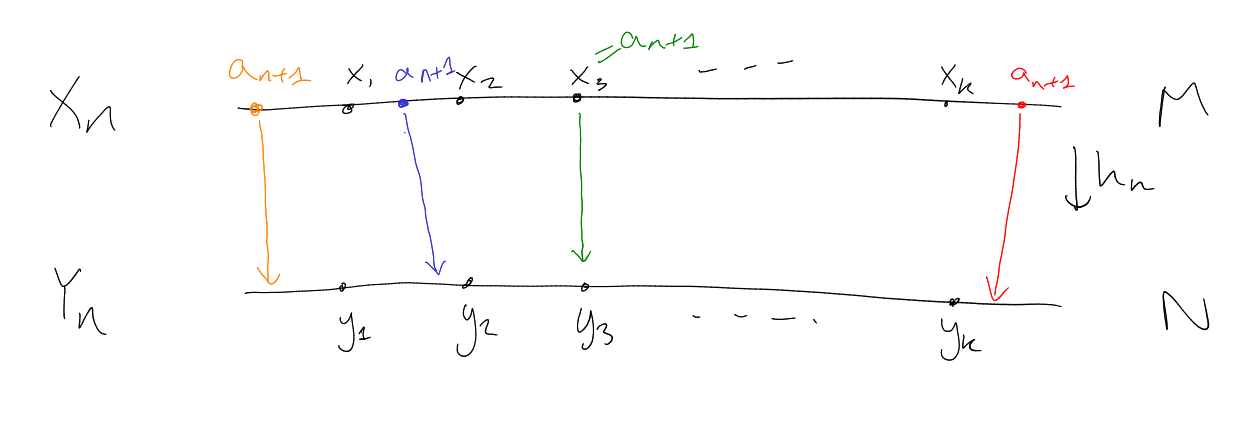
We will use the back and forth method.

Let $M = {a_{1}, a_{2}, \dots}$ and $N = {b_{1}, b_{2}, \dots}$ .

We construct a series of functions ${(h_{n})}_{n = 0}^{\infty}$ such that:

(i) $h_{n} : X_{n} \to Y_{n}$ is an order-preserving bijection.
(ii) $X_{n} \subseteq X_{n + 1}, Y_{n} \subseteq Y_{n + 1}, h_{n} \subseteq h_{n + 1}$ for each $n$ .
(iii) $a_{n} \in X_{n}$ , $b_{n} \in Y_{n}$ .

Once we have done this, $h = ⋃_{n = 0}^{\infty} h_{n}$ is an order-preserving bijection $h : M \to N$ (i.e. an $L$ -isomorphism).

Use induction.

Base case: $X_{0} = {x_{0}}$ , $Y_{0} = {b_{0}}$ , $h_{0} (a_{0}) = b_{0}$ .

Inductive step: Suppose $h_{n} : X_{n} \to Y_{n}$ as required.

“Forth”: Construct an order preserving bijection $h_{*} : X_{*} \to Y_{*}$ extending $h_{n}$ with $a_{n + 1} \in X_{*}$ . Enumerate $X_{n} = {x_{1}, \dots, x_{k}}$ with $x_{1} <^{M} x_{2} <^{M} x_{3} <^{M} \dots <^{M} x_{k}$ . Let $y_{i} = h (x_{i})$ so that $y_{1} <^{M} y_{2} <^{M} \dots <^{M} y_{k}$ .

Define $h_{*} = h_{n} \cup {(a_{n + 1}, b)}$ where $b \in N$ is chosen according to the following cases:

If $a_{n + 1} = x_{i}$ for some $i \in {1, \dots, k}$ , then put $b = x_{i}$ .
If $a_{n + 1} < x_{i}$ for all $i \in {1, \dots, k}$ then choose $b$ such that $b < y_{i}$ for all $i \in {1, \dots, k}$ (possible since no endpoints).
If $x_{i} < a_{n + 1}$ for all $i \in {1, \dots, k}$ , then choose $b$ such that $y_{i} < b$ for all $i \in {1, \dots, k}$ (possible since no endpoints).
If there is some $i \in {1, \dots, k - 1}$ such that $x_{i} < a_{n + 1} < x_{i + 1}$ , then choose $b$ such that $y_{i} < b < y_{i + 1}$ (possible since $M$ is dense).

Then $h_{*}$ is an order-preserving bijection and $a_{n + 1} \in X_{n + 1}$ as desired.

“Back”: We need to construct an order-preserving map $h_{n + 1} \to Y_{n + 1}$ extending $h_{*}$ with $b_{n + 1} \in Y_{n + 1}$ .

Exercise.

Then $h_{n + 1}$ satisfies the conditions. □

Note. We used that $N, M$ were countable.

The theory DLO is not uncountably categorical:

Consider $(ℝ, <)$ , and consider $ℝ \times ℚ$ with the lexicographic order ( $(a, b) < (c, d)$ if and only if $a < c$ or $a = c$ and $b < d$ ). These are both models of DLO (and have the same cardinality), but are not isomorphic (e.g. because the first does not have any countable intervals, or because the second does not have all bounded suprema).

Corollary 3.5. DLO is complete.

Proof. No finite models (because of the no end points axiom).

If $M, N ⊨ DLO$ , with both countable, then $M ≅ N$ and hence $M \equiv N$ .

So by Los-Vaught test, DLO is complete. □

4 Filters

Definition 4.1 (Filter). Let $J$ be a set. A filter $F$ on $J$ is a non-empty subset of $P (J)$ such that:

$\emptyset \notin F$ .
$\forall A, B \in F, A \cap \in F$ (“closed under finite intersections”).
$\forall A \in F$ , if $A \subseteq B \subseteq B \subseteq J$ , then $B \in F$ (“closed under super set”).

Example 4.2.

For $J$ infinite,
$F : = {A \subseteq J : J ∖ A is finite}$

is a filter.

For $J$ non-empty, and any $i \in J$ ,

F = {A \subseteq J : i \in J}

is a filter.

Definition 4.3 (Ultrafilter). Let $J$ be an infinite set and $F$ a filter on $J$ . We say $F$ is an ultrafilter if every filter $G$ on $J$ satisfying $F \subseteq G$ also satisfies $G = F$ .

Proposition 4.4. Assuming that:

$J$ a set
$F$ a filter on $J$

Then

F

is an ultrafilter if and only if for every

A \subseteq J

either

A \in F

J ∖ A \in F

Proof. Example Sheet 1. □

Proposition 4.5. Assuming that:

$J$ is a set
$F$ a filter on $J$

Then there is an ultrafilter

U

such that

F \subseteq U

Proof (sketch). Let $X$ be the set of filters extending $F$ , and partially order it by inclusion. Note every chain has an upper bound (take the union), so by Zorn’s lemma we have a maximal element, which is a ultrafilter (by definition). □

5 Ultraproducts

Definition 5.1. Let ${(A_{j})}_{j \in J}$ be a family of sets ( $J \neq \emptyset$ ), with $A_{j} \neq \emptyset$ for all $j \in J$ . Take $J$ to be an ultrafilter on $J$ , and define the following equivalence relation $\sim$ on $\prod_{j \in J} A_{j}$ :

{(a_{j})}_{j \in J} \sim {(b_{j})}_{j \in J} iff {j \in J : a_{j} = b_{j} \in U} .

Proposition 5.2. The relation $\sim$ defined above is an equivalence relation on $\prod_{j \in J} A_{j}$ .

Proof. Symmetric / reflexive is obvious.

Transitivity: let ${(a_{j})}_{j \in J}, {(b_{j})}_{j \in J}, {(c_{j})}_{j \in J} \in \prod_{j \in J} A_{j}$ , and suppose ${(a_{j})}_{j \in J} \sim {(b_{j})}_{j \in J}$ and ${(b_{j})}_{j \in J} \sim {(c_{j})}_{j \in J}$ .

Let

\begin{array}{l} F_{a b} & = {j \in J : a_{j} = b_{j}} \\ F_{b c} & = {j \in J : b_{j} = c_{j}} \\ F_{a c} & = {j \in J : a_{j} = c_{j}} \end{array}

Note $F_{a b}, F_{b c} \in U$ . Also,

\underset{\in U}{\underset{⏟}{F_{a b} \cap F_{b c}}} = {j \in J : a_{j} = b_{j} = c_{j}} \subseteq F_{a c}

hence $F_{a c} \in U$ , i.e. ${(a_{j})}_{j \in J} \sim {(c_{j})}_{j \in J}$ . □

Definition 5.3. Let ${(A_{j})}_{j \in J}$ be a non-empty family of non-empty sets and $U$ an ultrafilter on $J$ .

Write $\prod_{j \in J} A_{j} ∕ U$ to be $\prod_{j \in J} A_{j} ∕ \sim$ (where $\sim$ is defined as in Definition 5.1).
${[{(a_{j})}_{j \in J}]}_{U}$ is the equivalence class of ${(a_{j})}_{j \in J}$ with respect to $\sim$ .
Let $B_{j} \subseteq A_{j}$ for every $j \in J$ . Then
${[{(B_{j})}_{j \in J}]}_{U} = {[{(a_{j})}_{j \in J}] \in \prod_{j \in J} A_{j} ∕ U : {j \in J : a_{j} \in B_{j}} \in U} .$

Is the third item well-defined?

Proposition 5.4. Assuming that:

${(A_{j})}_{j \in J}$ , ${(B_{j})}_{j \in J}$ satisfy $B_{j} \subseteq A_{j}$ for all $j$
${(a_{j})}_{j \in J}, {(b_{j})}_{j \in J} \in \prod_{j \in J} A_{j}$ satisfying ${(a_{j})}_{j \in J} \sim {(b_{j})}_{j \in J}$

Then

{j \in J : a_{j} \in B_{j}} \in U

if and only if

{j \in J : b_{j} \in B_{j}} \in U

Proof. Know ${(a_{j})}_{j \in J} \sim {(b_{j})}_{j \in J}$ . Define

\begin{array}{l} U & = {j \in J : a_{j} = b_{j}} \in U \\ V & = {j \in J : a_{j} \in B_{j}} \\ W & = {j \in J : b_{j} \in B_{j}} \end{array}

Note $U \cap V \subseteq W$ and $U \cap W \subseteq V$ .

If $V \in U$ then $U \cap V \in U$ so $W \in U$ . Similarly, if $W \in U$ then $V \in U$ . □

So $[{(B_{j})}_{j \in J}]$ is well-defined.

Proposition 5.5. Assuming that:

${(A_{j})}_{j \in J}$ , $U$ , $\sim$ as usual.
$B_{j}, C_{j} \subseteq A_{j}$

Then

(1) $[{(B_{j})}_{j \in J}] \cap [{(C_{j})}_{j \in J}] = [{(B_{j} \cap C_{j})}_{j \in J}]$ .
(2) $[{(B_{j})}_{j \in J}] \cup [{(C_{j})}_{j \in J}] = [{(B_{j} \cup C_{j})}_{j \in J}]$ .
(3) $[{(B_{j})}_{j \in J}] ∖ [{(C_{j})}_{j \in J}] = [{(B_{j} ∖ C_{j})}_{j \in J}]$ .

Proof. Example Sheet 1. □

Definition 5.6. Let ${(A_{j})}_{j \in J}$ , $U$ (ultrafilter on $J$ ), $\sim$ as before, and let $n \in ℕ$ .

For each $j \in J$ , suppose $B_{j} \subseteq A_{j}^{n}$ . Define

\begin{array}{l} [{(B_{j})}_{j \in J}] & = {([{(a_{j}^{1})}_{j \in J}], \dots, [{(a_{j}^{n})}_{j \in J}]) \in {(\prod_{j \in J} A_{j} ∕ U)}^{n} : {j \in J : (a_{j}^{1}, \dots, a_{j}^{n}) \in B_{j}} \in U} \\ \subseteq {(\prod_{j \in J} A_{j} ∕ U)}^{n} \end{array}

Note. If $n = 0$ , then we get that

\begin{array}{l} B_{j} & = {()} \\ [{(B_{j})}_{j \in J}] & = {()} \end{array}

Definition 5.7. Let $n > 0$ , $k \in {1, \dots, n}$ . Define:

$π_{k} (x_{1}, \dots, x_{n}) = (x_{1}, \dots, x_{k - 1}, x_{k + 1}, \dots, x_{n})$ .
For $X$ a set of $n$ -tuples,

$π_{k} (X) = {(x_{1}, \dots, x_{k - 1}, x_{k + 1}, \dots, x_{n}) : (x_{1}, \dots, x_{n}) \in X} .$

Proposition 5.8. Assuming that:

${(A_{j})}_{j \in J}$ , $U$ , $\sim$ as usual
$n \in ℕ$
for each $j$ we have $B_{j}, C_{j} \subseteq A_{j}^{n}$

Then

(1) $[{(B_{j})}_{j \in J}] \cap [{(C_{j})}_{j \in J}] = [{(B_{j} \cap C_{j})}_{j \in J}]$
(2) $[{(B_{j})}_{j \in J}] \cup [{(C_{j})}_{j \in J}] = [{(B_{j} \cup C_{j})}_{j \in J}]$
(3) $[{(B_{j})}_{j \in J}] ∖ [{(C_{j})}_{j \in J}] = [{(B_{j} ∖ C_{j})}_{j \in J}]$

(4) If

n > 0

k \in {1, \dots, n}

then

π_{k} ([{(B_{j})}_{j \in J}]) = [{(π_{k} (B_{j}))}_{j \in J}] .

Proof. (1) - (3): Straightforward. See Example Sheet.

(4): Let $n > 0$ , $k \in {1, \dots, n}$ . Let

α = ([{(a_{j}^{1})}_{j \in J}], \dots, [{(a_{j}^{k - 1})}_{j \in J}], [{(j_{j}^{k + 1})}_{j \in J}], \dots, [{(a_{j}^{n})}_{j \in J}]) \in π_{k} ([{(B_{j})}_{j \in J}]) .

So we have some $[{(a_{j}^{k})}_{j \in J}]$ such that

([{(a_{j}^{1})}_{j \in J}], \dots, [{(a_{j}^{n})}_{j \in J}]) \in [{(B_{j})}_{j \in J}] .

So $U = {j \in J : (a_{j}^{1}, \dots, a_{j}^{n}) \in B_{j}} \in U$ .

Consider

V = {j \in J : (a_{j}^{1}, \dots, a_{j}^{k - 1}, a_{j}^{k + 1}, \dots, a_{n}) \in π (B_{j})} \supseteq U .

So $α \in [{(π_{k} (B_{j}))}_{j \in J}]$ , i.e. $π_{k} [{(B_{j})}_{j \in J}] \subseteq [{(π_{k} (B_{j}))}_{j \in J}]$ .

Showing $[{(π_{k} (B_{j}))}_{j \in J}] \subseteq π ([{(B_{j})}_{j \in J}])$ is similar (do it as an exercise). □

Definition 5.9. Suppose $A_{j} = A$ for each $j \in J$ . Then we call $\prod_{j \in J} A_{j} ∕ U$ an ultrapower of $A$ , and write $A^{U}$ .

If $B \subseteq A$ , we write $[B]$ for $[{(B)}_{j \in J}]$ .

Theorem 5.10. Assuming that:

$A^{U}$ be as above
$J = ℕ$
${C \subseteq ℕ : ℕ ∖ C is finite} \subseteq U$
$n \in ℕ$
for each m ∈ ℕ, let Bm ⊆ An satisfying:
- (1) $[B_{m}] \neq \emptyset \forall m \in ℕ$
- (2) $[B_{k}] \subseteq [B_{m}]$ for all $m, k \in ℕ$ with $m \leq k$

Then

⋂_{m \in ℕ} [B_{m}] \neq \emptyset

Proof. Omitted. For $n = 1$ , this is a potential presentation topic. □

6 Ultraproduct Structures

Definition 6.1. Let $M_{j} = (M_{j}, I_{j})$ be $L$ -structures for each $j \in J$ . Let $U$ be an ultraproduct on $J$ . Define an interpretation $I_{U}$ of $L$ on $\prod_{j \in J} M_{j} ∕ U$ . Let $S \in L$ .

S

is an

n

-ary relation:

I_{U} (S) = [{(I_{j} (S))}_{j \in J}] \subseteq {(\prod_{j \in J} M_{j} ∕ U)}^{n} .

If $S$ is a constant:
$I_{U} (S) = [{(I_{j} (S))}_{j \in J}] \in \prod_{j \in J} M ∕ U .$

Functions are a bit less clear. However, we can always turn a function into a relation by looking at its graph (i.e.

f : M^{n} \to M

has graph

R_{f} = {(\bar{x}, y) \in M^{n + 1} : f (\bar{x}) = y}

So if $S$ is a function: for each $j \in J$ , define the graph of $I_{j} (S)$ as

G_{j} (S) = {(a_{1}, \dots, a_{n}, b) \in M_{j}^{n + 1} : I_{j} (S) (a_{1}, \dots, a_{n}) = b} .

Then $[{(G_{j} (S))}_{j \in J}]$ is the graph of a function

{(\prod_{j \in J} M_{j} ∕ U)}^{n} \to \prod_{j \in J} M_{j} ∕ U .

(Checking this is left as an exercise). Now define $I_{U} (S)$ to be the function corresponding to $[{(G_{j} (S))}_{j \in J}]$ .

Example 6.2. $L = {+, R}$ (where $+$ is a function and $R$ is a unary relation). Let $C_{n} = (C_{n}, I_{n})$ with $C_{n} = ℤ ∕ n ℤ$ , with addition modulo $n$ , and let $I_{n} (R) = {x \in C_{n} : \exists y \in C_{n}, 2 y = x}$ .

Consider $C = (\prod_{n \in ℕ_{> 0}} C_{n} ∕ U, I_{U})$ .

What does the set $I_{U} (R)$ look like?

If $\gcd (n, 2) = 1$ , then $I_{n} (R) = C_{n}$ .

If $\gcd (n, 2) = 2$ , then $I_{n} (R) \neq C_{n}$ (for example, $1 \notin I_{n} (R)$ ).

If $U = {A \subseteq ℕ : 3 \in A}$ , then $C ≅ C_{3}$ , so $I_{U} (R) = C$ .
Homework: Can you think of two non-principal ultrafilters, with one of them having $I_{U} (R) = C$ , and the other having $I_{U} (R) \neq C$ .

Options to think about:

(a) Every $U \in U$ contains an even number.
(b) Every $U \in U$ contains an odd number.
(c) There is a $U \in U$ all even.
(d) There is a $U \in U$ all odd.

Consider $b = (1, 1, 1, \dots) \in \prod_{n \in ℕ} C_{n}$ .

Suppose (a), so for every $K \in U$ we have $i \in K$ even, i.e. $b_{i} \notin I_{R} (C_{1})$ , so $I_{R} (C) \neq C$ . Note (a) is equivalent to (c).

By similar reasoning, (b) implies $I_{R} (C) = C$ (and also (b) is equivalent to (c)).

7 Łoś’s Theorem and Consequences

Question, how does $φ (\prod_{j \in J} M_{j} ∕ U)$ relate to $[φ {(M_{j})}_{j \in J}]$ ?

Theorem 7.1 (Los Lemma). Assuming that:

$L$ a language
$φ$ an $L$ -formula
${(M_{j})}_{j \in J} = {(M_{j}, I_{j})}_{j \in J}$ a non-empty family of $L$ -structures
$U$ an ultrafilter on $J$
$M = (\prod_{j \in J} M_{j} ∕ U, I_{U})$

Then

φ (M) = [φ {(M_{j})}_{j \in J}] .

Proof (sketch). Induction on

Complexity of terms
Formulas

(essentially Proposition 5.8). □

Corollary 7.2. Assuming that:

$σ$ an $L$ -sentence
${(M_{j})}_{j \in J}$ a family of non-empty $L$ -structures
$U$ an ultrafilter on $J$
$M = \prod_{j \in J} M_{j} ∕ U$

Then

M ⊨ σ

if and only if

{j \in J : M_{j} ⊨ σ} \in U

Proof.

$\Rightarrow$ Suppose $M ⊨ σ$ . Then $σ (M)$ is a non-empty subset of $M^{0}$ , i.e. its the empty tuple (). So ${[{(σ (M_{j}))}_{j \in J}]} = {()}$ . So
${j \in J : () \in σ (M_{j})} = {j \in J : M_{j} ⊨ σ} .$

Since the LHS is in $U$ , we get that the RHS is too.
$\Leftarrow$ Similar □

Theorem 7.3 (Compactness – ultraproduct proof). Assuming that:

$L$ a language
$Σ$ a set of $L$ -sentences

Then

Σ

is consistent if and only if every finite subset of

Σ

is consistent.

Proof.

$\Rightarrow$ Clear.
$\Leftarrow$ Assume every finite subset of $Σ$ is consistent. Let $J$ be the set of all finite subsets of $Σ$ . For each $j \in J$ , let
$ĵ = {k \in J : j \subseteq k} .$

Let $B = {ĵ : j \in J}$ and let
$F = {A \subseteq J : \exists B \in B, B \subseteq A} .$

Exercise: $F$ is a filter.

Let $U$ be an ultrafilter extending $F$ . For each $j \in J$ , let $M_{j} ⊨ j$ . Let $M = (\prod_{j \in J} M_{j} ∕ U)$ .

Claim: $M ⊨ Σ$ .

Let $σ \in Σ$ . Then ${σ} \in J$ and $\hat{{σ}} \subseteq {j \in J : M_{j} ⊨ σ}$ .

So ${j \in J : M_{j} ⊨ σ} \in U$ , so $M ⊨ σ$ .

So: $\forall σ \in Σ, M ⊨ σ$ . □

8 More Constructions

Let $L$ be a language, $M$ an $L$ -structure. Fix a collection ${(M_{i})}_{i \in I}$ of substructures of $M$ . Let $N = ⋂_{i \in I} M_{i}$ , and assume $N$ is non-empty.

Then we have a canonical $L$ -structure, with universe $N$ and interpretiation:

For $f$ a function, $f^{N} = f^{μ} |_{N}$ (which equals $f^{M_{i}} |_{N}$ for each $i \in I$ )
For $R$ an $n$ -ary relation, $R^{N} = R^{M} \cap N^{n}$ (which equals $R^{M_{i}}$ for each $i \in I$ )
For $c$ a constant, $c^{N} = c^{M}$ (which equals $c^{M_{i}}$ for each $i \in I$ )

Note $N$ is also a substructure.

Definition 8.1 (Generated by). Given an $L$ -structure $M$ , a non-empty $A \subseteq M$ , the substructure generated by $A$ is the intersection of all substructures containing $A$ .

Definition 8.2 (Chain, Elementary chain). Let $α$ be a limit ordinal.

A collection ${(M_{i})}_{i < α}$ of $L$ -structures is a chain if $M_{i} \subseteq M_{j}$ (substructure) for all $i < j$ , and is an elementary chain if $M_{i} ≼ M_{j}$ for all $i < j$ .

If ${(M_{i})}_{i < α}$ is a chain then $⋃_{i < α} M_{j}$ is a well-defined $L$ -structure.

9 Algebraically closed fields

Definition (Algebraically closed). Suppose $(K, +, \cdot)$ is a field (in $L_{rings}$ ). It is algebraically closed if every non-constant polynomial over $K$ has a root in $K$ .

Definition 9.1 (ACF). $ACF$ is the $L_{rings}$ theory axiomatising algebraically closed fields. It consists of:

field axioms
for every $d \geq 1$ , we add an axiom:
$\forall v_{0}, \dots, v_{d}, \exists x (v_{d} \neq 0 ⟹ v_{0} + v_{1} x + \dots + v_{d} x^{d} = 0) .$

Note. This is an infinite axiomatisation.

Definition 9.2 (ACF with characteristic). For $n \geq 1$ , let $χ_{n}$ be the sentence

\underset{n times}{\underset{⏟}{1 + \dots + 1}} = 0 .

Set

\begin{array}{l} {ACF}_{0} & = ACF \cup {\neg χ_{n} : n \in ℕ} \\ {ACF}_{p} & = ACF \cup {χ_{p}} & (for p a prime) \end{array}

Theorem 9.3. ${ACF}_{0}$ and ${ACF}_{p}$ are $κ$ -categorical for $κ > ℵ_{0}$ .

Proof. The Transcendence degree of $k ⊨ ACF$ (and algebraically closed field) is the cardinality of the largest algebraically independent subset of $k$ .

For example,

\begin{array}{l} {trdeg}_{ℚ} (\bar{ℚ}) & = 0 \\ {trdeg}_{ℚ} (\bar{ℚ (π)}) & = 1 \\ {trdeg}_{ℚ} (ℂ) & = 2^{ℵ_{0}} \\ {trdeg}_{ℚ} (\bar{ℚ {(x_{i})}_{i < κ}}) & = κ \end{array}

From algebra we know:

(1) If k,k′⊨ACF ⁡ then k≅k′ if and only if
- $trdeg (k) = trdeg (k^{'})$
- $char (k) = char (k^{'})$
- $| k | = | k^{'} |$
(2) If $k ⊨ ACF$ , $λ = {trdeg}_{ℚ} (k)$ , then $| κ | = ℵ_{0} + λ$ . Thus if $k, k^{'} ⊨ {ACF}_{0}$ or ${ACF}_{p}$ are uncountable and $| k | = | k^{'} |$ then ${trdeg}_{ℚ} (k) = {trdeg}_{ℚ} (k^{'})$ so $k ≅ k^{'}$ . □

Corollary 9.4. ${ACF}_{0}$ and ${ACF}_{p}$ are complete.

Proof. Los-Vaught test. □

Remark. ${ACF}_{0}$ and ${ACF}_{p}$ are not $ℵ_{0}$ -categorical. (Consider fields with different finite transcendence degrees).

Definition 9.5 (Polynomial map). Let $k$ be a field. We say a function $ϕ : K^{m} \to K^{m}$ is a polynomial map if

Φ (\bar{x}) = (p_{1} (x_{1}, \dots, x_{m}), \dots, p_{n} (x_{1}, \dots, x_{m}))

where each $p_{1}, \dots, p_{n}$ is a polynomial.

Theorem 9.6 (Ax-Grothendieck). Assuming that:

$k$ an algebraically closed field
$Φ : K^{n} \to K^{n}$ an injective polynomial map

Then

Φ

is surjective.

Proof. First suppose $K = \bar{𝔽_{p}}$ for some prime $p$ . $\bar{𝔽_{p}} = ⋃_{k} 𝔽_{p^{k}}$ . Fix an $m$ such that the coefficients of $Φ$ all lie in $𝔽_{p^{m}}$ . Note: $\bar{𝔽_{p}} = ⋃_{k} 𝔽_{p^{m k}}$ .

For any $k \geq 1$ , $Φ$ induces an injective polynomial map $𝔽_{p^{k m}} \to 𝔽_{p^{k m}}$ which has to be surjective (as finite field). Hence

\begin{array}{l} Φ ({\bar{𝔽_{p}}}^{n}) & = Φ (⋃_{k} 𝔽_{p^{m k}}^{n}) \\ = ⋃_{k} Φ (𝔽_{p^{m k}}^{n}) \\ = ⋃_{k} 𝔽_{p^{m k}}^{n} \\ = {\bar{𝔽_{p}}}^{n} \end{array}

So $Φ$ is surjective.

Given $n, d \geq 1$ , let $ψ_{n, d}$ be the $L$ -sentence expressing “every injective polynomial map with $n$ -coordinates, each of which is a polynomial in $n$ variables with degree at most $d$ , is surjective”.

Exercise: Show that this is a first order $L_{rings}$ sentence.

Now $\bar{𝔽_{p}} ⊨ ψ_{n, d}$ for all $n, d \geq 1$ and $p$ prime.

${ACF}_{p}$ is complete, so ${ACF}_{p} ⊨ ψ_{n, d}$ . Now consider ${ACF}_{0}$ . Suppose for contradiction that ${ACF}_{0} ⁄ ⊨ ψ_{n, d}$ for some $n, d$ , so ${ACF}_{0} ⊨ \neg ψ_{n, d}$ .

By compactness, there exists $Σ \subseteq {ACF}_{0}$ finite such that $Σ ⊨ \neg ψ_{n, d}$ .

In particular, $Σ \subseteq ACF \cup {\neg χ_{0}, \dots, \neg χ_{m}}$ for some $m$ . Choose a prime $p$ such that $p > m$ and ${ACF}_{p} ⊢ Σ$ .

So must have ${ACF}_{p} ⊨ \neg ψ_{n, d}$ , contradiction. □

Theorem 9.7 (Lipschiptz principal). Assuming that:

$ϕ$ an $L_{rings}$ sentence

Then the following are equivalent:

(1) ${ACF}_{0} ⊨ ϕ$ , i.e. $ϕ$ in every $k ⊨ {ACF}_{0}$
(2) ${ACF}_{0} \cup {ϕ}$ is consistent
(3) there exists some $n > 0$ such that ${ACF}_{p} ⊨ ϕ$ for any $p > n$
(4) for all $n > 0$ , there exists some $p > n$ such that ${ACF}_{p} \cup {ϕ}$ is consistent

10 Diagrams

Let $N, M$ be $L$ -structures.

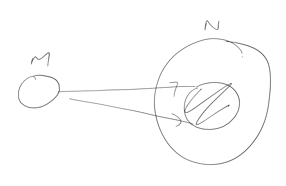
Remark 10.1. If $h : M \to N$ is an (elementary) $L$ -embedding then after identifying $a \in M$ with $h (a) \in N$ we can view $M$ as an (elementary) substructure of $N$ .

Given $A \subseteq M$ , let $L_{A} = L \cup {\underset{̲}{a} : a \in A}$ where $\underset{̲}{a}$ is a new constant symbol. Then $M$ is an $L_{A}$ -structure. Interpret $\underset{̲}{a}$ as $a$ .

Definition 10.2 (Diagram). The diagram of $M$ (respectively elementary diagram), $D (M)$ , is the set of quantifier-free $L_{M}$ -sentences (respectively all $L_{M}$ -sentences) true in $M$ .

Proposition 10.3. Assuming that:

$M$ is an $L$ -structure
$N^{*}$ an $L_{M}$ -structure such that $N^{*} ⊨ D (M)$
let $N$ be the $L$ -reduct of $N^{*}$ to $L$ (means throw away $L_{M} ∖ L$ sentences)
define $h : M \to N$ such that $h (a) = \underset{̲}{a} = a^{N}$ .

Then

h

is an

L

-embedding. Moreover, if

N^{*} ⊨ {T h}_{M} (M)

then

h

is an elementary

L

-embedding.

Proof. We use Corollary 2.4. Let $φ (x_{1}, \dots, x_{n})$ be a quantifier-free $L$ -formula, and fix $a_{1}, \dots, a_{n} \in M$ . Then

\begin{array}{l} M ⊨ φ (a_{1}, \dots, a_{n}) & ⟺ φ (\underset{̲}{a_{1}}, \dots, \underset{̲}{a_{n}}) \in D (M) \\ ⟺ N^{*} ⊨ φ (\underset{̲}{a_{1}}, \dots, \underset{̲}{a_{n}}) \\ ⟺ N ⊨ φ (h (a_{1}), \dots, h (a_{n})) \end{array}

Therefore $h$ is an $L$ -embedding.

“Moreover” is similar. □

Remark. You can use this to show that any torsion free abelian group is orderable ( Example Sheet 2).

11 Introduction to Quantifier Elimination

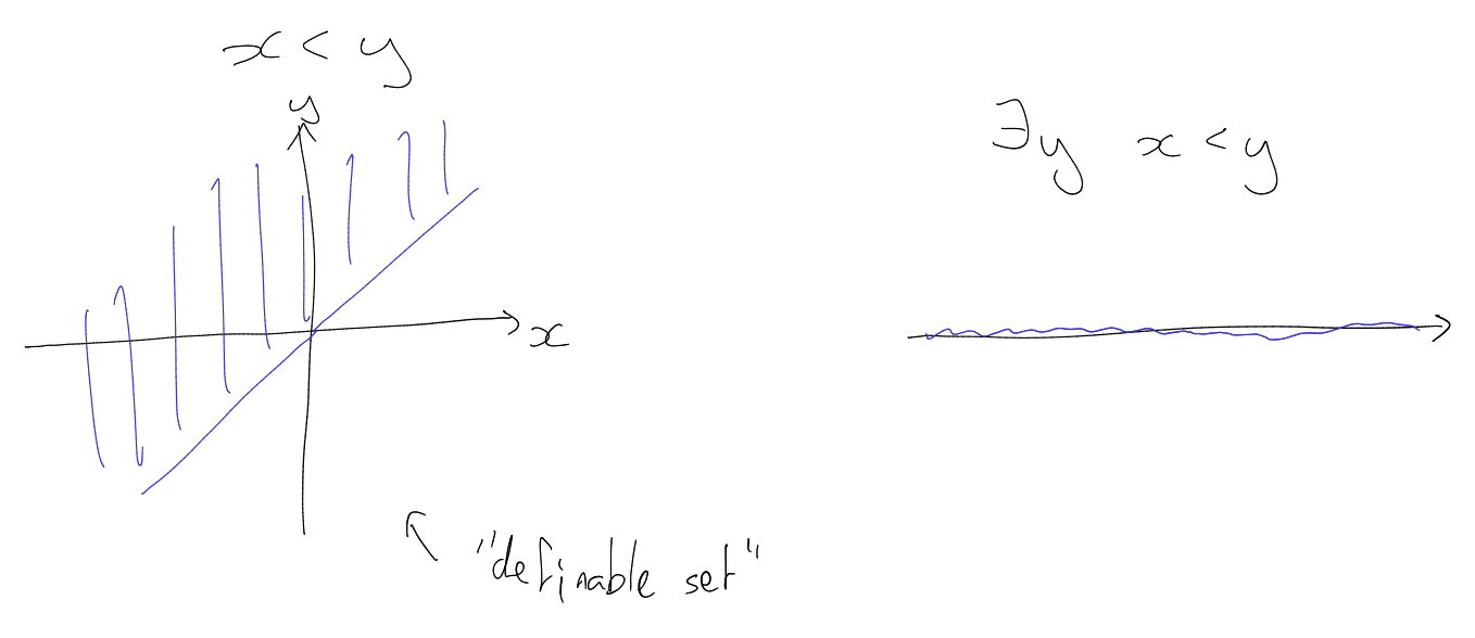
Definition (Definable set). Let $T$ be an $L$ -theory and $M ⊨ T$ . Then $X \subseteq M^{n}$ is definable is there is some $L$ -formula $φ (x_{1}, \dots, x_{n})$ such that

X = {\bar{a} \in M^{n} : M ⊨ φ (\bar{a})} .

Definition 11.1 (Theory has quantifier elimination). An $L$ -theory $T$ has quantifier elimination (QE) if for any $L$ -formula $φ (x_{1}, \dots, x_{n})$ ther eis a quantifier free formula $ψ (x_{1}, \dots, x_{n})$ such that

T ⊨ \forall \bar{x} (φ (\bar{x}) \leftrightarrow ψ (\bar{x})) .

(i.e. they define the same set in all models).

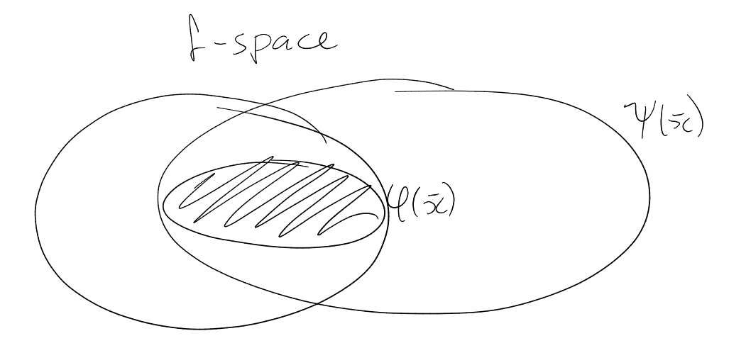
Example 11.2.

(1) Let

T = T h (F)

F

a field in

L_{rings}

. Let

φ (w, x, y, z)

be the formula saying

“ (\begin{matrix} w & x \\ y & z \end{matrix}) has an inverse”,

i.e.

\exists s, t, u, v [(\begin{matrix} s & t \\ u & v \end{matrix}) (\begin{matrix} w & x \\ y & z \end{matrix}) = (\begin{matrix} 1 & 0 \\ 0 & 1 \end{matrix})] .

Then

T ⊨ \forall x, w, y, z (φ (w, x, y, z) ⟺ w z - x y \neq 0) .

(2) Let $T = T h (ℝ, \cdot, +, 0, 1)$ . Consider $φ (x) = \exists y (y^{2} = x)$ (this defines $ℝ_{\geq 0}$ ).
Quantifier free formulas in one variable are boolean combinations of polynomial equations, i.e. define sets of size finite or cofinite. But $ℝ^{\geq 0}$ is infinite-co-infinite, so cannot be defined by a quantifier free formula.

Remark: $T h (ℝ, \cdot, +, 0, 1)$ does have quantifier elimination.

We can show $T h (ℝ, \cdot, +, 0, 1)$ and $T h (ℝ, \cdot, +, 0, 1, <)$ have the same definable sets.

This is because we can define $<$ in $L_{rings}$ in $T$ by noting $x < y$ if and only if
$\exists z (z \neq 0 \land y - z^{2} = x) .$

Note: you can always find a language in which the theory of a structure has quantifier elimination: just add a relation symbol for each non quantifier-free formula. This is called the “Morleyisation” of a structure, but isn’t particularly informative.

Lemma 11.3. Assuming that:

$T$ is an $L$ -theory
for any quantifier-free formula $φ (x_{1}, \dots, x_{n}, y)$ there is a quantifier-free formula $ψ (x_{1}, \dots, x_{n})$ such that
$T ⊨ \forall \bar{x} (\exists y φ (\bar{x}, y) \leftrightarrow ψ (\bar{x})) .$

Then

T

has quantifier elimination.

Proof. Exercise: induction on the complexity of formulas. □

Theorem 11.4. Assuming that:

$T$ an $L$ -theory

Then the following are equivalent:

(i) $T$ has quantifier elimination
(ii) Let $M, N ⊨ T$ , $A \subseteq M$ , $A \subseteq N$ (substructures). For any quantifier-free formula $φ (x_{1}, \dots, x_{n}, y)$ and tuple $\bar{a} \in A$ , if $M ⊨ \exists y, φ (\bar{a}, y)$ then $N ⊨ \exists y, φ (\bar{a}, y)$ .
(iii) For any $L$ -structure $A$ , $T \cup D (A)$ is a complete $L_{A}$ -theory.

Proof.

(i)

⟹

(iii) Assume

T

has quantifier elimination, and let

A

be an

L

-structure. Suppose

M, N ⊨ T \cup D (A)

. We want to show

M \equiv_{L_{A}} N

Let $σ$ be an $L_{A}$ -sentence, and suppose that $M ⊨ σ$ . Then $σ$ can be written as $φ (\bar{a})$ where $φ (\bar{x})$ is an $L$ -formula and $\bar{a} \in A$ .

By quantifier elimination, we have $ψ (\bar{x})$ such that

T ⊨ \forall \bar{x} (φ (\bar{x}) \leftrightarrow ψ (\bar{x})) .

Now $M ⊨ T$ , so $M ⊨ \forall \bar{x} (φ (\bar{x}) \leftrightarrow ψ (\bar{x}))$ , and $M ⊨ φ (\bar{a})$ . So $M ⊨ ψ (\bar{a})$ . Now $ψ (\bar{a}) \in D (A)$ as $M ⊨ D (A)$ . So $N ⊨ ψ (\bar{a})$ , as $N ⊨ D (A)$ . Hence $N ⊨ φ (\bar{a})$ as $N ⊨ T$ (i.e. $N ⊨ \forall \bar{x} (φ (\bar{x}) \leftrightarrow ψ (\bar{x}))$ ). So $N ⊨ σ$ .

(iii) $⟹$ (ii) Let $M, N ⊨ T$ , $A \subseteq M$ , $A \subseteq N$ . Let $φ (\bar{x}, y)$ be a quantifier free formula and let $\bar{a} \in A$ such that $M ⊨ \exists y φ (\bar{a}, y)$ .
As $A \subseteq M$ , $A \subseteq N$ , we have $M, N ⊨ T \cup D (A)$ , so by (iii) we have $M \equiv_{L_{A}} N$ so $N ⊨ \exists φ (\bar{a}, y)$ .

(ii)

⟹

(i) We want to show quantifier elimination.

By Lemma 11.3, it is sufficient to show for $φ (\bar{x}, y)$ quantifier free, we can find $ψ (\bar{x})$ quantifier free such that

T ⊨ \forall \bar{x} (\exists y, φ (\bar{x}, y) \leftrightarrow ψ (\bar{x})) .

Let $L^{*} = L \cup {c_{1}, \dots, c_{n}}$ where each $c_{i}$ is a new constant (with $n = | \bar{x} |$ ). Let

Γ = {ψ (\bar{x}) : ψ (\bar{x}) quantifier free formula such that T ⊨ \forall \bar{x}, (\exists y, φ (\bar{x}, y) \to ψ (\bar{x}))} .

In definable sets:

Claim: $T \cup Γ ⊨ \exists y, φ (\bar{x}, y)$ .

Proof: Suppose not. Then there is an $L^{*}$ -structure

N ⊨ T \cup Γ \cup {\neg \exists y, φ (𝜀, y)} .

Let $a_{i} = c_{i}^{N}$ , and let $A \subseteq N$ be the substructure generated by $a_{1}, \dots, a_{n}$ in $N$ .

Then $N ⊨ T$ , $A \subseteq N$ , $N ⊨ \neg \exists y, φ (\bar{c}, y)$ . Any $b \in A$ is of the form $t^{N} (\bar{a})$ for an $L$ -term $t$ (exercise).

So $D (A)$ can be viewed as an $L^{*}$ -structure by replacing $\underset{̲}{b}$ ( $b = t^{N} (\bar{a})$ ) with $t (\bar{c})$ in $L^{*}$ . Let

Σ = T \cup D (A) \cup {\exists y, φ (\bar{x}, y)} .

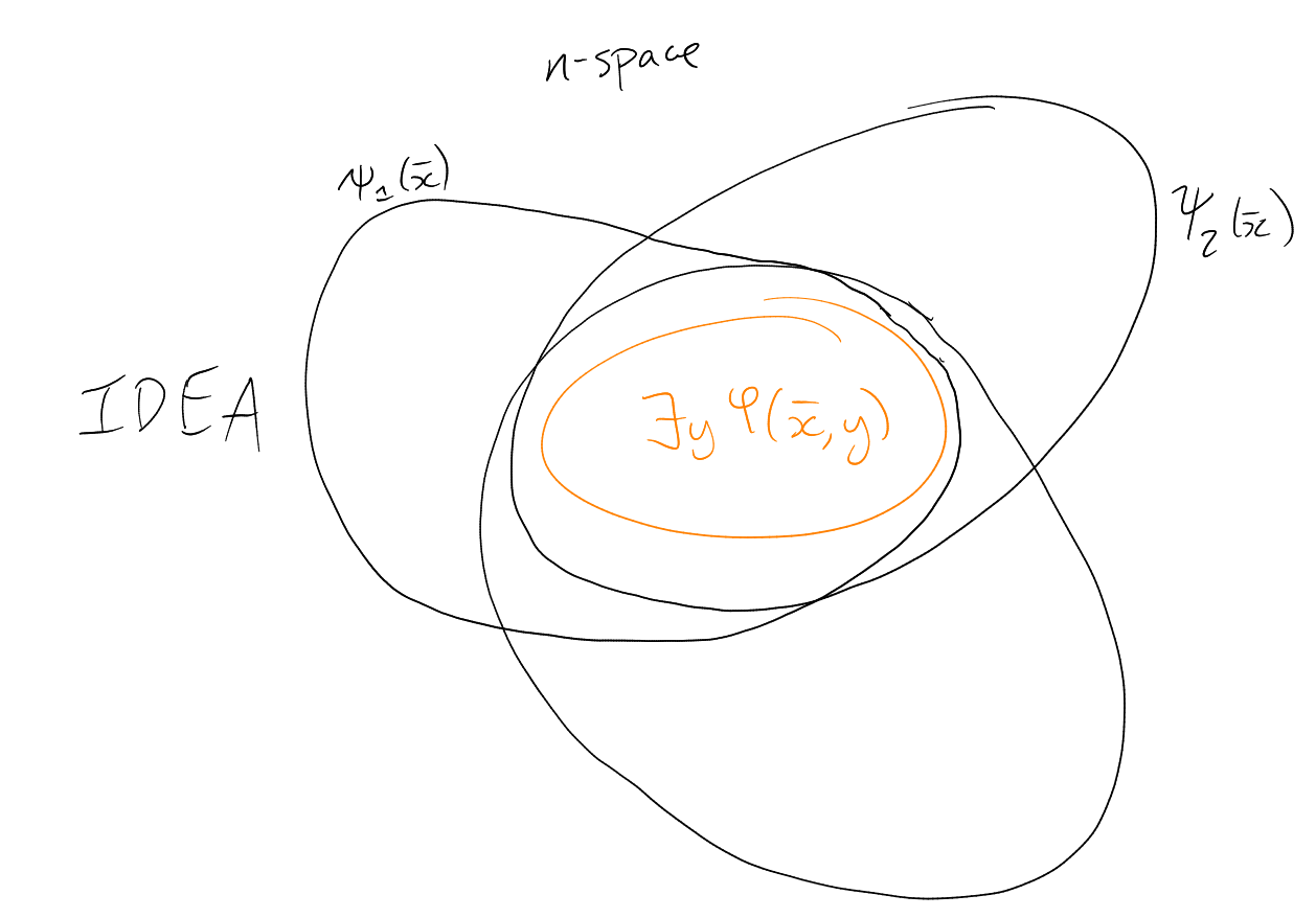
IDEA: build $M ⊨ Σ$ , $M ⊨ T \cup D (A)$ and $M ⊨ \exists y, φ (\bar{a}, Y)$ , contradicting (ii).

Suffices to prove $Σ$ is consistent.

Assume $Σ$ is inconsistent. Then by compactness we have $ψ_{1} (\bar{x}), \dots, ψ_{n} (\bar{x})$ quantifier free $L$ -formulas with

$ψ_{1} (\bar{c}), \dots, ψ_{m} (\bar{c}) \in D (A)$ .
$T \cup {\land_{i = 1}^{m} ψ_{i} (\bar{c})} \cup {\exists y, φ (\bar{c}, y)}$ is unsatisfiable.

In definable sets:

Let $ψ (\bar{x})$ be $\neg \land_{i = 1}^{m} ψ_{i} (\bar{x})$ , then $T ⊨ \exists y, φ (\bar{c}, y) \to ψ (\bar{c})$ .

So $T ⊨ \forall \bar{x} (\exists y, φ (\bar{x}, y) \to ψ (\bar{x}))$ so $ψ (\bar{c}) \in Γ$ . So $N ⊨ ψ (\bar{c})$ but also $N ⊨ D (A)$ ( $A \subseteq N$ ). Then

N ⊨ \underset{\in D (A)}{\underset{⏟}{\land_{i = 1}^{m} ψ_{i} (\bar{c})}} = \neg ψ (\bar{c})

contradiction. So by compactness, $Σ$ is consistent.

This proves the claim.

Reminder: the claim was that $T \cup Γ ⊨ \exists y, φ (\bar{x}, y)$ . So by compactness, there are $ψ_{1} (\bar{x}), \dots, ψ_{m} (\bar{x})$ quantifier free such that

T \cup \underset{\subseteq Γ}{\underset{⏟}{{ψ (\bar{c}), \dots, ψ_{m} (\bar{c})}}} ⊨ \exists y, φ (\bar{x}, y) .

Recall

T ⊨ \forall \bar{x} (\exists y, φ (\bar{x}, y) \to \land_{i = 1}^{m} ψ_{i} (\bar{x}))

by choice of $n$ . Let

ψ (\bar{x}) = \land_{i = 1}^{m} ψ_{i} (\bar{x}) .

Then

T ⊨ ψ (\bar{c}) \to \exists y, φ (\bar{c}, y)

hence

T ⊨ \forall \bar{x} (ψ (\bar{x}) \to \exists y, φ (\bar{x}, y)) .

Thus $T ⊨ \forall \bar{x}, (ψ (\bar{x}) \leftrightarrow \exists y, φ (\bar{x}, y))$ . □

Remark.

(1) In (iii) we may assume $A \subseteq M ⊨ T$ , as otherwise $T \cup D (A)$ is inconsistent and hence trivially complete.
(2) In (ii) and (iii) we may assume $A$ is finitely generated.

12 Examples

Theorem 12.1. $ACF$ has quantifier elimination.

Proof. We will show that condition Theorem 11.4(iii) holds.

So we need to show that for any finitely generated $A$ , $T \cup D (A)$ is complete.

Fix a finitely generated $L$ -structure $A$ and show $ACF \cup D (A)$ is complete. Use Los-Vaught test. Fix $K_{1}, K_{2} ⊨ ACF \cup D (A)$ uncountable, wiht $| K_{1} | = | K_{2} |$ . $A$ is a finitely generated integral domain contained in $K_{1}, K_{2}$ .

So since $A$ contains $1$ , it determines the characteristic. So $char (K_{1}) = char (K_{2})$ . So $K_{1} ≅ K_{2}$ (in $L_{rings}$ ).

Need an $L_{A}$ -isomorphism, i.e. an isomorphism $Φ : K_{1} \to K_{2}$ preserving $A$ . Consider $F_{i}$ the fraction field of $A$ in $K_{i}$ . The field of fractions of an integral domain is unique up to isomorphism, i.e. $\exists τ : F_{1} \to F_{2}$ preserves $A$ pointwise.

$A$ is finitely generated (hence finite $trdeg$ ), so $trdeg (K_{1} ∕ F_{1}) = trdeg (K_{2} ∕ F_{2})$ . Therefore $τ$ extends to $τ^{*} : K_{1} \to K_{2}$ fixing $A$ pointwise. So $K_{1} ≅_{L_{A}} K_{2}$ . □

Definition 12.2 (Constructible). Let $F$ be a field. We say that $X \subseteq F^{n}$ is constructible if it is a boolean combination of subsets of $F^{n}$ defined by $p (x_{1}, \dots, x_{n}) = 0$ for $p (\bar{x}) \in F [\bar{x}]$ .

Corollary 12.3 (Chevalley’s Theorem). Assuming that:

$K ⊨ ACF$
$X \subseteq K^{n}$ a constructible set

Then the projection

Y = {(a_{1}, \dots, a_{n - 1}) \in K^{n - 1} : (\bar{a}, b) \in X for some b \in K}

of $X$ is also constructible.

Definition 12.4 (Rado graph). Let $L = {E}$ , with $E$ a binary relation. A Rado or Random graph is a graph $(V, E)$ such that $V \neq \emptyset$ and for any finite disjoint $X, Y \subseteq V$ there is some $v \in V$ such that:

$E (v, x)$ for all $x \in X$
$\neg (v, y)$ for all $y \in Y$

We denote the theory of Rado graphs as $R C$ . It consists of

Graph axioms (irreflexive and symmetric).

For any $k \geq 1$ and $l \geq 1$ ,

\forall x_{1}, \dots, x_{k}, \forall y_{1}, \dots, y_{l} (\underset{i, j}{\land} x_{i} \neq y_{j} \to \exists v (\underset{i, j}{\land} E (v, x_{i}) \land \neg E (v, y_{j}))) .

Facts:

$R G$ is $ℵ_{0}$ -categorical.
If $M ⊨ R G$ then every finite graph is an induced subgraph.
Suppose $M, N ⊨ R G$ are two coutnable models, and $f : X \to Y$ is a graph isomorphism between $X \subseteq M$ (finite) and $Y \subseteq M$ (finite). Then $f$ extends to an isomorphism from $M$ to $N$ .

Theorem 12.5. $R G$ has quantifier elimination.

Proof. Option 1: Show $R G \cup D (A)$ , with $A$ a finite graph is complete.

Option 2: Use (ii) of Theorem 11.4. Fix $M, N ⊨ R G$ , $A \subseteq M \cap N$ . Fix a quantifier-free formula $φ (x_{1}, \dots, x_{n}, y)$ , $\bar{a} \in A^{n}$ . Assume that there exists $b \in M$ , $M ⊨ φ (\bar{a}, b)$ . Want to show $\exists c \in N$ such that $N ⊨ φ (\bar{a}, c)$ .

Write $φ (\bar{x}, y)$ in disjunction normal form:

\lor_{s = 1}^{k} \land_{t = 1}^{l_{s}} 𝜃_{s, t} (\bar{x}, y)

where $𝜃_{s, t} (\bar{x}, y)$ is atomic or negated atomic. There is some $s \subseteq k$ such that $M ⊨ \land_{t = 1}^{l_{s}} 𝜃_{s, t} (\bar{a}, b)$ .

Each of $𝜃_{s, t} (\bar{x}, y)$ is one of $x_{i} = x_{j}$ , $x_{i} = y$ , $E (x_{i}, x_{j})$ , $E (x_{i}, y)$ and negations.

If $x_{i} = y$ appears then $b = a_{i} \in A \subseteq N$ and so $N ⊨ φ (\bar{a}, b)$ .

We may assume $x_{i} = y$ does not appear in $𝜃_{s, t}$ . Let

\begin{array}{l} X & = {a_{i} : M ⊨ E (a_{i}, b)} \subseteq \bar{a} \\ Y & = {a_{i} : M ⊨ \neg E (a_{i}, b)} \subseteq \bar{a} \end{array}

Then $X$ and $Y$ are finite and disjoint. So we have $c \in N$ such that

\begin{array}{l} N & ⊨ E (a_{i}, c) \forall a_{i} \in X \\ N & ⊨ \neg E (a_{i}, c) \forall a_{i} \in Y \\ c & \notin {a_{i}, \dots, a_{n}} \end{array}

So $N ⊨ \land_{t = 1}^{l_{s}} 𝜃_{s, t} (\bar{a}, c)$ and thus $N ⊨ φ (\bar{a}, c)$ . □

13 Introduction to Types

Definition ( $L$ -formula with parameters from $A$ ). Given a language $L$ , an $L$ -structure $M$ and a subset $A \subseteq M$ , we call an $L_{A}$ -formula an $L$ -formula with parameters from $A$ .

Write these as $φ (\bar{x}, \bar{a})$ for $φ (\bar{x}, \bar{y})$ an $L$ -formula, and $\bar{a} \in A$ (identify with ${\underset{̲}{a}}^{M}$ ).

Suppose $N ≽ M$ . What does $N$ look like from the point of $M$ ?

SIngle formulas don’t give you much insight: suppose $a \in N$ , $N ⊨ ϕ (a)$ . Then there is some $a^{'} \in M$ with $M ⊨ ϕ (a^{'})$ .

This changes if you consider sets of infinitely many formulas.

Notation 13.1.

Let $p$ be a set of formulas in free variables $x_{1}, \dots, x_{n}$ . We often write $\underset{̲}{p (x_{1}, \dots, x_{n})}$ and $\underset{̲}{p}$ interchangeably.
Given $M$ and $a_{1}, \dots, a_{n} \in M$ , we write $M ⊨ p (a_{1}, \dots, a_{n})$ if $M ⊨ ϕ (a_{1}, \dots, a_{n})$ for every $ϕ \in p$ .
We say $p$ is consistent if it is realised in some $L$ -structure.

Exercise: Show $p$ is consistent if and only if every finite subest of $p$ is consistent ( Example Sheet 2, Q8).

Definition 13.2 ( $n$ -type). Let $M$ be an $L$ -structure and $A \subseteq M$ . An $n$ -type over $A$ with respect to $M$ is a set of $L$ -formulas with parameters from $A$ , in free variables $x_{1}, \dots, x_{n}$ such that $p \cup {T h}_{A} (M)$ is consistent.

An $n$ -type is complete if for every $L_{A}$ -formula with $n$ variables $ϕ$ , either $ϕ \in p$ or $\neg ϕ \in p$ .

Let $S_{n}^{M} (A)$ denote the set of all complete $n$ -types over $A$ with respect to $M$ .

Definition 13.3 ( $t p^{M}$ ). Given $a_{1}, \dots, a_{n} \in M$ , let ${t p}^{M} (a_{1}, \dots, a_{n} ∕ A)$ be the set of all $L_{A}$ -formulas $ϕ (x_{1}, \dots, x_{n})$ such that $M ⊨ ϕ (a_{1}, \dots, a_{n})$ (usually $a_{i} \notin A$ ).

${t p}^{M} (\bar{a} ∕ A) \in S_{n}^{M} (A)$ and $\bar{a} ⊨ {t p}^{M} (\bar{a} ∕ A)$ .

Proposition 13.4. Assuming that:

$p \in S_{n}^{M} (A)$

Then there is

N ≽ M

with

\bar{a} \in N^{n}

such that

p = {t p}^{N} (\bar{a} ∕ A)

Proof. By assumption $p \cup {T h}_{A} (M)$ is consistent.

Need to show $p \cup {T h}_{M} (M)$ is consistent.

Fix $Σ \subseteq p \cup {T h}_{M} (M)$ finite. $Σ \subseteq p \cup {φ_{1}, \dots, φ_{t}}$ , $φ_{i}$ an $L_{M}$ -sentence with $M ⊨ φ_{i}$ .

Let $φ^{*}$ be $\land_{i = 1}^{t} φ_{i}$ , then $φ^{*}$ can be written $φ^{*} (b_{1}, \dots, b_{m})$ where $b_{1}, \dots, b_{m} \in M ∖ A$ and $φ^{*} (x_{1}, \dots, x_{m})$ an $L_{A}$ -formula.

Since $M ⊨ φ^{*} (b_{1}, \dots, b_{m})$ we get $M ⊨ \exists \bar{v}, φ^{*} (v_{1}, \dots, v_{m})$ , so $\exists \bar{v} φ^{*} (\bar{v}) \in {T h}_{A} (M)$ .

So as ${T h}_{A} (M) \cup p$ is consistent, we have $N ⊨ {T h}_{A} (M) \cup p$ with

$\bar{c} \in N^{m}$ with $N ⊨ φ^{*} (\bar{c})$ .
$\bar{a} \in N^{m}$ with $N ⊨ p (\bar{a})$ .

Expand $N$ to an $L_{M}$ -structure, i.e. let

$b_{i}^{N} = c_{i}$ for $i \in {1, \dots, m}$ .
${\bar{b}}^{N}$ arbitary for $b \in M ∖ ⟨ (A \cup {b_{1}, \dots, b_{m}}) ⟩$ .

Then $N ⊨ φ (b_{1}, \dots, b_{m})$ . So $N ⊨ φ^{*}$ , so $N ⊨ Σ$ . □

Remark 13.5. If $M ≼ N$ and $A \subseteq M$ then $S_{n}^{M} (A) = S_{n}^{N} (A)$ since ${T h}_{A} (M) = {T h}_{A} (N)$ .

Remark 13.6. $p$ is an $n$ -type over $A$ with respect to $M$ if and only if $\forall q \subseteq p$ finite, $\exists \bar{a} \in M^{n}$ such that $\bar{a} ⁄ ⊨ q$ .

Proof.

$\Rightarrow$ Clear.
$\Leftarrow$ Choose $N ≽ M$ realising $p$ . Fix $q \subseteq p$ finite, $φ (\bar{x})$ the conjunction of all $L_{A}$ -formulas in $q$ . Then $N ⊨ \exists \bar{x}, φ (\bar{x})$ . So $M ⊨ \exists \bar{x}, φ (\bar{x})$ , i.e. $q$ is realised in $M$ . □

Example 13.7. Suppose $K ⊨ ACF$ , $A \subseteq K$ . We want to describe $S_{n}^{K} (A)$ . Fix $p \in S_{n}^{K} (A)$ . By quantifier elimination we only need to consider quantifier free formulas.

Moreover,

\begin{array}{l} φ \land ψ \in p & ⟺ φ, ψ \in p \\ \neg ψ \in p & ⟺ φ \notin p \end{array}

So we can concentrate on atomic formulas $φ$ , polynomials in variables $x_{1}, \dots, x_{n}$ over the field generated by $A$ , say $F$ (i.e. $F [\bar{x}]$ ).

Let $I_{p} = {f (\bar{x}) \in F [\bar{x}] : f (\bar{x}) = 0 \in p}$ . Then $I_{p}$ is a prime ideal and $p \mapsto I_{p}$ is a bijection $S_{n}^{K} (A) \mapsto Spec F [\bar{x}]$ ( $Spec F [\bar{x}]$ is the set of prime ideals of $F [\bar{x}]$ ). So $S_{1}^{K} (A)$ consists of

{p_{a} : a \in A} \cup {q},

where $p_{a}$ contains (and thus is determined by) $x = a$ and $q = {x \neq a : a \in F}$ .

$| S_{1}^{K} (K) | = | K |$ .

14 Type Spaces

Definition. Let $M$ be an $L$ -structure, $A \subseteq M$ . Given an $L_{A}$ -formula $φ (x_{1}, \dots, x_{n})$ , define

[φ (x_{1}, \dots, x_{n})] = {p \in S_{n}^{M} (A) : φ (x_{1}, \dots, x_{n}) \in p} .

We have the following basic properties:

(i) $S_{n}^{M} (A) = [\land_{i = 1}^{n} x_{i} = x_{i}]$ .
(ii) $[φ (\bar{x}) \land φ (\bar{x})] = [φ (\bar{x})] \cap [ψ (\bar{x})]$ .
(iii) $[\neg φ (\bar{x})] = S_{n}^{M} (A) ∖ [φ (\bar{x})]$ .

We define a topology on $S_{n}^{M} (A)$ (“the logic topology”) by taking $[φ (\bar{x})]$ for all $L_{A}$ -formulas $φ (\bar{x})$ as a basis of open sets.

Theorem 14.1. $S_{n}^{M} (A)$ is a totally disconnected compact Hausdorff space.

Proof. Showing that it is a topology is left as an exercise.

Hausdorff: Fix $p, q \in S_{n}^{M} (A)$ distinct. Then there is a $φ (\bar{x})$ $L_{A}$ -formula such that $φ (\bar{x}) \in p$ and $\neg φ (\bar{x}) \in q$ . Then $p \in [φ (\bar{x})]$ and $q \in [\neg φ (\bar{x})]$ – these are disjoint.

Compactness: Sufficient to consider open covers consisting of basic open sets. SUppose we have $L_{A}$ -formulas ${(φ_{i} (\bar{x}))}_{i \in I}$ such that $S_{n}^{M} (A) = ⋃_{i \in I} [φ_{i} (\bar{x})]$ . Let $Σ = {\neg φ_{i} (\bar{x}) : i \in I}$ .

Claim: $Σ \cup {T h}_{A} (M)$ is inconsistent.

Proof of claim: Otherwise $N ⊨ {T h}_{A} (M)$ , $\bar{a} \in N^{n}$ such that $\bar{a} ⊨ Σ$ . Let $p = {t p}^{N} (\bar{a} ∕ A) \in S_{n}^{M} (A)$ . But $p \notin [φ_{i} (\bar{x})] \forall i \in I$ , contradiction.

So by compactness we have finite $I_{0} \subseteq I$ with

{\neg φ_{i} (\bar{x}) : i \in I_{0}} \cup {T h}_{A} (M) (∗)

inconsistent.

Claim: $S_{n}^{M} (A) = ⋃_{i \in I_{0}} [φ_{i} (\bar{x})]$ .

Proof: Fix $p \in S_{n}^{M} (A)$ . We can realise $p$ in some $N ⊨ {T h}_{A} (M)$ , i.e. we have $\bar{a} \in N^{n}$ with $\bar{a} ⊨ p$ .

By ( $*$ ), we have $N ⊨ φ_{i} (\bar{a})$ for some $i \in I_{0}$ . So $φ_{i} (\bar{x}) \in p$ , so $p \in [φ_{i} (\bar{x})]$ .

Totally disconnected: In a compact Hausdorff space, we have totally disconnected if and only if two points are separated by a clopen set. All basic sets are clopen, so totally disconnected. □

15 Saturated Models

Definition 15.1. Let $M$ be an infinite $L$ -structure, and $κ > | L | + ℵ_{0}$ . We say $M$ is $κ$ -saturated if for any $A \subseteq M$ with $| A | < κ$ , every type in $S_{n}^{M} (A)$ is realised in $M$ for all $n$ .

Remark 15.2.

(i) Restricting to complete types is not important, as every $n$ -type over $A$ with respect to $M$ can be extended to a complete type.
(ii) It suffices to assume $n = 1$ to prove $κ$ -saturation.
(iii) If $M$ is $κ$ -saturated then $| M | \geq κ$ . ${x \neq a : a \in M}$ is a consistent $1$ -type over $M$ in $M$ .

Definition 15.3 (Partial elementary / homogeneous). Let $M, N$ be $L$ -structures, $A \subseteq M$ , $B \subseteq N$ . A function $f : A \to B$ is partial elementary if for every $L$ -formulas $φ (x_{1}, \dots, x_{n})$ and $a_{1}, \dots, a_{n} \in A$ we have

M ⊨ φ (\bar{a}) ⟺ N ⊨ φ (f (\bar{a})) .

Given $κ \geq | L | + ℵ_{0}$ , $M$ is $κ$ -homogeneous if for any $A \subseteq M$ with $| A | < κ$ , any partial elementary map $f A \to M$ and any $c \in M$ there is some $d \in M$ with $f \cup {(c, a)}$ partial elementary. In other words, “partial elementary maps can be extended”.

For the rest of this section, assume $T$ to be a complete $L$ -theory with infinite models.

Definition 15.4. Define $S_{n} (T) = S_{n}^{M} (\emptyset)$ for any / some $M ⊨ T$ (because if $M, N ⊨ T$ , then $S_{n}^{N} (\emptyset) = S_{n}^{M} (\emptyset)$ as $T h (M) = T h (N) = T$ ).

Proposition 15.5. Assuming that:

$T$ a complete $L$ -theory with infinite models
$M ⊨ T$

Then

M

ℵ_{0}

-saturated if and only if

M

ℵ_{0}

-homogeneous and

M

realises all types in

S_{n} (T)

n \geq 1

Proof.

$\Rightarrow$ Assume $M$ is $ℵ_{0}$ -saturated. In particular, $M$ realises all types in $S_{n} (T)$ ( $\emptyset$ is finite).
Fix some finite $A \subseteq M$ , and a partial elementary map $f : A \to M$ . (Aim: find $d \in M$ such that $f \cup {(c, d)}$ is partial elementary). Given $c \in M$ , define $p \in S_{1}^{M} (f (A))$ to be such that
$φ (x, f (\bar{a})) ⟺ M ⊨ φ (c, \bar{a})$

(for all $φ (y, \bar{x})$ $L$ -formulas and $\bar{a} \in A$ ). Write $p = f ({t p}^{M} (c ∕ \bar{a}))$ .

To show $p \in S_{1}^{M} (f (A))$ , consider $φ (x, \bar{a}) \in p$ . Then $M ⊨ φ (c, \bar{a})$ , so $M ⊨ \exists x, φ (x, \bar{a})$ , os $M ⊨ \exists φ (x, f (\bar{a}))$ as $f$ is partial elementary.

So $p$ is finitely satisfiable, and completeness follows from ${t p}^{M} (c ∕ A)$ being complete. So as $M$ is $κ$ -saturated we have $d ⊨ p$ for some $d \in M$ . Then $f \cup {(c, d)}$ is a partial elementary map.
$\Leftarrow$ Fix $a_{1}, \dots, a_{n} \in M$ , $p \in S_{1}^{M} ({a_{1}, \dots, a_{n}})$ . We want to show $p$ is realised in $M$ .
Set
$q = {φ (y, x_{1}, \dots, x_{n}) : φ (y, \bar{a}) \in p} \in S_{n + 1}^{M} (T) .$

So by assumption, we have $d, b_{1}, \dots, b_{n}$ with $(d, \bar{b}) ⊨ q$ .

Consider $t p (\bar{a} ∕ \emptyset) = t p (\bar{b} ∕ \emptyset)$ . So $f : b_{i} \to a_{i}$ is partial elementary. Let $c \in M$ such that $f \cup {(d, c)}$ is partial elementary. Then ${t p}^{M} (c, \bar{a}) = {t p}^{M} (d, \bar{b})$ . So $(c, \bar{a}) ⊨ q$ and $t p (c ∕ \bar{a}) = p$ . □

Notation. Given $M$ , $\bar{a}, \bar{b} \in M^{n}$ , write $\bar{a} \equiv^{M} \bar{b}$ if ${t p}^{M} (\bar{a}) \equiv^{M} \bar{b}$ .

So $M$ is $ℵ_{0}$ -homogeneous if and only if whenever $\bar{a} \equiv^{M} \bar{b}$ and $c \in M$ , there exists $d \in M$ with $\bar{a} c \equiv^{M} \bar{b} d$ .

Lemma 15.6. Assuming that:

$T$ a complete $L$ -theory with infinite models
$M ⊨ T$

Then there is an

N ≽ M

with

| N | \leq | M | + | L |

and

N

ℵ_{0}

-homogeneous.

Proof. First claim: For any $M ⊨ T$ , there is $N ≽ M$ with $| N | \leq | M | + | L |$ and for any $\bar{a}, \bar{b}, c$ from $M$ such that $\bar{a} \equiv^{M} \bar{b}$ there is some $d \in N$ with $\bar{a} c \equiv^{N} \bar{b} d$ .

Proof of claim: Enumerate all $(\bar{a}, \bar{b}, \bar{c})$ as ${({\bar{a}}_{α}, {\bar{b}}_{α}, {\bar{c}}_{α})}_{α \leq | M |}$ . Now let $M_{0} = M$ , and use transfinite induction to form a chain ${(M_{α})}_{α < | M |}$ .

$α$ is a limit ordinal: set $M_{α} = ⋃_{i < α} M_{i}$ (then $| M_{α} | \leq | α | (| M | + | L |) = | M | + | L |$ as $α \leq | M |$ ).
Given $α$ (not a limit ordinal), look at $(a_{α}, b_{α}, c_{α})$ . Assume ${\bar{a}}_{α} \equiv^{M_{α}} {\bar{b}}_{α}$ so $f_{α} : {\bar{a}}_{α} \to {\bar{b}}_{α}$ partial elementary. Then we apply Proposition 13.4 (Note the elementary super structure construnted here is of size $\leq | M | + | L |$ ) to find $M_{α + 1} ≽ M_{α}$ with $| M_{α + 1} | \leq | M_{α} | + | L | \leq | M | + | L |$ with a $d \in M_{α + 1}$ realising $f_{α} (t p (c_{α} ∕ a_{α}))$ . Then by construction, $({\bar{a}}_{α} c) \equiv^{M_{α + 1}} ({\bar{b}}_{α} d)$ .

Now let $N = ⋃_{α < | M |} M_{α}$ . Note that we might have introduced new elements. Note $| N | \leq | M | (| M | + | L |) = | M | + | L |$ .

We build a new chain $M = N_{0} ≼ N_{1} ≼ N_{2} ≼ \dots$ of countably many steps with $| N_{1} | \leq | M | + | L |$ and such that for any $\bar{a}, \bar{b}, \bar{c} \in N$ , if $\bar{a} \equiv^{M} \bar{b}$ then there is $d \in N_{i + 1}$ such that $\bar{a} c \equiv^{N_{i + 1}} \bar{b} d$ . We do this by iterating the claim.

FInally let $N = ⋃_{i < ℵ_{0}} N_{i}$ . Then:
- $| N | \leq | M | + | L |$ .
- $N$ is $ℵ_{0}$ -homogeneous as any $\bar{a}, \bar{b}, c$ from $N$ lie in $N_{i}$ for some $i$ .

□

Definition 15.7 (Saturated). We say $M$ is saturated if it is $| M |$ -saturated.

Theorem 15.8. Assuming that:

$T$ a complete $L$ -theory with infinite models
$L$ is countable

Then

T

has a countable saturated model if and only if

S_{n} (T)

is countable for every

n \geq 1

Proof.

$\Rightarrow$ M⊨T countable, saturated.
- $M^{n}$ is countable for all $n \in ℕ$ .
- We have a map $p \to \bar{a} ⊨ p$ ( $p \in S_{n} (T)$ , $\bar{a}$ some realisation). This is map since $M$ saturated, and injective (because complete types).
So $S_{n} (T)$ is countable.
$\Leftarrow$ Enumerate $⋃_{n \geq 1} S_{n} (T) = {p_{1}, p_{2}, p_{3}, \dots}$ . Fix a countable $M_{0} ⊨ T$ , and build a chain $M_{0} ≼ M_{1} ≼ M_{2} ≼ \dots$ such that $M_{i}$ realises $p_{i}$ and is countable, using Proposition 13.4.
Get $N = ⋃_{i \in ℕ} M_{i}$ . Then $N ⊨ T$ and is countable. $N$ realises all types over $\emptyset$ .

Apply Lemma 15.6 to get $M ≽ N$ countable and $ℵ_{0}$ -homogeneous structure.

So by Proposition 15.5 is is $ℵ_{0}$ -saturated. □

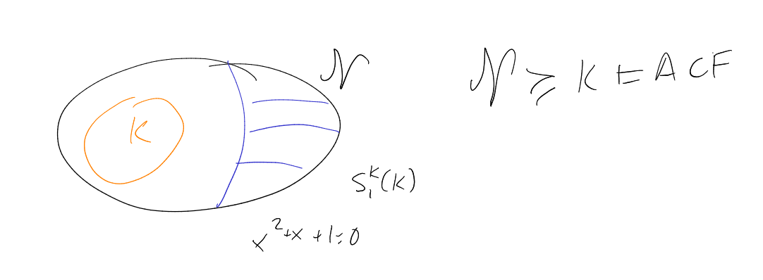
Example 15.9.

(i) Let $T = {ACF}_{p}$ and let
$F = {\begin{matrix} ℚ & if p = 0 \\ 𝔽_{p} & if p > \infty \end{matrix} .$

Then
$S_{n} (T) = Spec (F [x_{1}, \dots, x_{n}]) .$

Thus $S_{n} (T)$ is countable, since every ideal in $Spec (F [x_{1}, \dots, x_{n}])$ is finitely generated (Hilbert’s basis theorem). So by Theorem 15.8, ${ACF}_{p}$ has a countable saturated model which is the model of transcendence degree $ℵ_{0}$ .

Note: if $F ⊨ {ACF}_{p}$ has transcendence degree $n$ , the type determined by “ $x_{1}, \dots, x_{n + 1}$ ” is an algebraically independent set.
(ii) Let $T = T F D A G$ (torsion free, divisible abelian groups). This has a countable saturated model, which is the $ℚ$ -vector space of dimension $ℵ_{0}$ .
(iii) Let $T = T h (ℤ, +, 0)$ . For $n \geq 1$ , let $δ_{n} (x)$ be the $L$ -formula $\exists y (x = n y)$ , and let $ℙ$ be the set of primes. Given $X \subseteq ℙ$ finite,
$q_{x} = {δ_{n} (x) : n \in X} \cup {\neg δ_{n} (x) : n \in ℙ ∖ X} .$

$q_{X}$ is satisfiable in $ℤ$ , thus $\exists p_{X} \in S_{1} (T)$ with $q_{x} \leq p_{x}$ .

If $X \neq Y$ , then $p_{X} \neq p_{Y}$ , so $| S_{1} (T) | \geq 2^{ℵ_{0}}$ . By Theorem 15.8, $T$ doesn’t have a countable saturated model.

Example 15.10. Let $M ⊨ R G$ . We describe $S_{1}^{M} (M)$ . For $a \in M$ , let $p_{a} \in S_{1}^{M} (M)$ be the type containing “ $x = a$ ” (exercise: why is this unique).

FOr $V \leq M$ set

p_{V} = {x \neq a : a \in M} \cup {F (x, q) : a \in V} \cup {\neg E (x, a) : a \in M ∖ V} .

$p_{V}$ is a $1$ -type with respect to $M$ , not realised in $M$ , determines a complete $1$ -type, as we have determined all atomic formula, by $a \in p_{V}$ determines a complete type.

So $S_{1}^{M} (M) = {p_{a} : a \in M} \cup {p_{V} : V \subseteq M}$ .

$| S_{1}^{M} (M) | = 2^{| M |}$ .

Note: in general $| S_{1}^{M} (A) | \leq 2^{(| A | + | L | + ℵ_{0})}$ .

Proposition 15.11. Assuming that:

$T$ a complete $L$ -theory with infinite models
$M \equiv N$ are both countable and saturated

Then

M ≅ N

Proof. Exercise (use back and forth argument). □

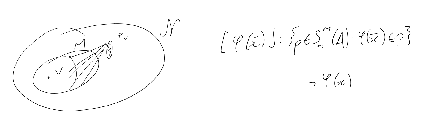
16 Omitting Types

Let $M$ be an $L$ -structure. Which types must be realised?

Definition 16.1. We say $p \in S_{n}^{M} (A)$ is isolated if it is an isolated point with respect to topology on $S_{n}^{M} (A)$ (i.e. ${p}$ is open).

Example. For $a \in A \subseteq M$ , ${t p}^{M} (a ∕ A)$ is isolated by $x = a$ ( ${{t p}^{M} (a ∕ M)} = [x = a]$ ).

Proposition 16.2. Assuming that:

$p \in S_{n}^{M} (A)$ .

Then the following are equivalent:

(i)
$p$ is isolated
(ii)
${p} = [φ (z)]$ for some $L_{A}$ -formula $φ (\bar{x})$ . In this case we say $φ (\bar{x})$ isolates $p$ .

(iii)

There is an

L_{A}

-formula

φ (\bar{x}) \in p

such that for any

ψ (\bar{x}) \in p

{T h}_{A} (M) ⊨ \forall x (φ (\bar{x}) \to ψ (\bar{x})) .

Proof. (i) $⟺$ (ii): Obvious.

(ii) $⟹$ (iii): Assume $φ (\bar{x})$ isolates $p$ . Fix an $L_{A}$ -formula $ψ (\bar{x})$ . We want to show $M ⊨ \forall \bar{x} (φ (\bar{x}) \to ψ (\bar{x}))$ . So suppose $M ⊨ φ (\bar{a})$ . Then ${t p}^{M} (\bar{a} ∕ A) \in [φ (\bar{x})] = {p}$ .

So ${t p}^{M} (\bar{a} ∕ A) = p$ , hence $M ⊨ ψ (\bar{a})$ .

(iii) $⟹$ (ii): By assumption, for every $L_{A}$ -formula we have $ψ (\bar{x}) \in p$ , $[φ (\bar{x})] \subseteq [ψ (\bar{x})]$ . Thus if $q \sin [φ (\bar{x})]$ , $a \in [ψ (\bar{x})]$ . So $ψ (\bar{x}) \in q$ , so $p \subseteq q$ , so $p = q$ . □

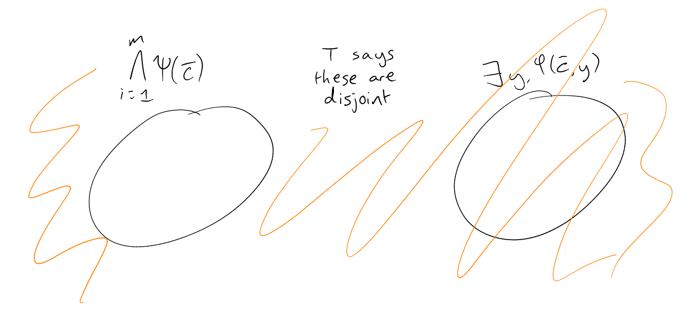
Proposition 16.3. Assuming that:

$T$ is complete and consistent
$p \in S_{n} (T)$ is isolated

Then

p

is realised in every

M ⊨ T

Proof. Fix $p \in S_{n} (T)$ , isolated by $φ (\bar{x})$ . Fix $M ⊨ T$ .

By Proposition 13.4, there is some $N ≽ M$ realising $p$ .

So $N ⊨ \exists \bar{x} φ (\bar{x})$ , so $M ⊨ \exists \bar{x} φ (\bar{x})$ .

Fix $\bar{a} \in M^{n}$ such that $M ⊨ φ (\bar{a})$ . Then $\bar{a} ⊨ p$ as for any $φ (\bar{x}) \in p$ we have

M ⊨ \forall \bar{x} (φ (\bar{x}) \to ψ (\bar{x})) .

So $M ⊨ φ (\bar{a})$ . □

Theorem 16.4 (Omitting Types Theorem). Assuming that:

$L$ is countable
$p \in S_{n} (T)$ is non-isolated

Then there is a countable

M ⊨ T

such that

p

is not realised in

M

(

M

omits

p

Proof. Let $L^{*} = L \cup C$ , with $C$ a countably infinite set of new constants.

An $L^{*}$ -theory has the witness property if for any $L^{*}$ -formula $φ (\bar{x})$ there is a constant $c \in C$ such that $T^{*} ⊨ \exists x φ (x) \to ψ (c)$ .

Fact: Suppose $T^{*}$ is a complete, satisfiable $L^{*}$ -theory with the witness property.

Define $\sim$ on $C$ such that $c \sim d$ if and only if $T^{*} ⊨ c = d$ . Let $M = C ∕ \sim$ , and define an $L^{*}$ -structure on $M$ such that:

$c^{M} = [c]$
$f^{M} ([c_{1}], \dots, [c_{n}]) = [d]$ if and only if
$T^{*} ⊨ f (c_{1}, \dots, c_{n}) = d .$
$R^{M} = {([c_{1}], \dots, [c_{n}]) \in M^{n} : T^{*} ⊨ R (c_{1}, \dots, c_{n})}$ .

Then $M$ is a well-defined $L^{*}$ -structure and $M ⊨ T^{*}$ .

Note we have $M ⊨ φ ([c_{1}], \dots, [c_{n}])$ if and only if $T^{*} ⊨ φ (c_{1}, \dots, c_{n})$ . We call $M$ the Henkin model of $T^{*}$ .

Fix $p \in S_{n} (T)$ non-isolated.

Aim: build a complete, satisfiable $L^{*}$ -theory $T^{*} \supseteq T$ , with the witness property, .

Such that for all $c_{1}, \dots, c_{n} \in C$ there is some $φ (\bar{x}) \in p$ such that $T^{*} ⊨ \neg φ (c_{1}, \dots, c_{n})$ . Then the Henkin model of $T^{*}$ omits $p$ .

Enumerate all the $L^{*}$ -sentences $φ_{0}, φ_{1}, \dots$ and all $c^{(} n = {{\bar{c}}_{1}, {\bar{c}}_{2}, \dots}$ . We build a satisfiable $L^{*}$ -theory $T \cup {𝜃_{1}, 𝜃_{2}, \dots}$ such that

(0) $⊨ 𝜃_{i} \to 𝜃_{j}$ for all $i > j$ .
(0) (Completeness): Either $⊨ 𝜃_{3 i + 1} \to φ_{i}$ or $⊨ 𝜃_{3 i + 1} \to \neg φ_{i}$ .
(0) (Witnessing property): If $φ_{i}$ is $\exists v ψ (v)$ for some $ψ$ and $⊨ 𝜃_{3 i + 1} \to φ_{i}$ then $⊨ 𝜃_{3 i + 2} \to ψ (c)$ for some $c$ . (check this does ensure the witness property).
(0) (Omit $p$ ): $⊨ 𝜃_{3 i + 3} \to \neg ψ (c_{i})$ for some $ψ (\bar{x}) \in p$ .

Let $𝜃_{0}$ be $\forall v (v = v)$ , and suppose we have $𝜃_{0}, \dots, 𝜃_{m}$ .

Case 1: $m + 1 = 3 i + 1$ for some $i$ .

If $T \cup {𝜃_{m}, φ_{i}}$ is satisfiable then $𝜃_{m + 1} = 𝜃_{m} \land φ_{i}$ . Otherwise $𝜃_{m + 1} = 𝜃_{m} \land \neg φ$ .

So $T \cup {𝜃_{m + 1}}$ is satisfiable by construction.

Case 2: $m + 1 = 3 i + 2$ for some $i$ .

Suppose $φ_{i}$ is $\exists v, ψ (v)$ for some $ψ$ an $L^{*}$ -formula, and $⊨ 𝜃_{i} \to φ_{i}$ (otherwise, let $𝜃_{m + 1} = 𝜃_{m}$ ).

Choose a $c \in C$ not used in $𝜃_{m}$ . Let $𝜃_{m + 1}$ be $𝜃_{m} \land ψ (i)$ .

Exercise: check $T \cup {𝜃_{m + 1}}$ is satisfiable.

Case 3: $m + 1 = 3 i + 3$ for some $i$ .

Let ${\bar{c}}_{i} = (c_{1}, \dots, c_{n})$ . Without loss of generality assume $x_{1}, \dots, x_{n}$ not used in $𝜃_{m}$ . We build an $L$ -formula as follows:

Replace $c_{t}$ by $x_{t}$ ( $t \in {1, \dots, n}$ ).
Replace any $c \in C ∖ {c_{1}, \dots, c_{n}}$ by new variables $v_{c}$ and add $\exists v_{c}$ to the front.

Then $φ (\bar{x})$ doesn’t isolated $p$ .

By Proposition 16.2, there is some $ψ (\bar{x}) \in p$ with

T ⁄ ⊨ \forall x (φ (\bar{x}) \to ψ (\bar{x})) .

Let $𝜃_{m + 1}$ be $𝜃_{m} \land \neg ψ (c_{1}, \dots, c_{n})$ . Check $𝜃_{m + 1}$ is satisfiable.

TODO □

Definition 16.5 (Atomic, prime). Fix $M ⊨ T$ .

We say $M$ is atomic if every $n$ -type over $\emptyset$ realised in $M$ is isolated.
We say $M$ is prime if for any $N ⊨ T$ there is an elementary embedding $M \to N$ .

Example. Let $K ⊨ {ACF}_{0}$ . Then $\bar{ℚ} = ℚ^{alg} \subseteq K$ , and $\bar{ℚ} < κ$ by quantifier elimination. So $\bar{ℚ}$ is the prime model of ${ACF}_{0}$ .

Assume $L$ is countable.

Fact: $M$ is prime if and only if $M$ is countable and atomic.

Theorem 16.6. Assuming that:

$L$ countable

Then the following are equivalent:

(i)
$T$ has a prime model.
(ii)
$T$ has an atomic model.
(iii)
For all $n \geq 1$ , the isolated types are dense.

Theorem 16.7.

(a)
Suppose $| S_{n} (T) | < 2^{ℵ_{0}}$ for all $n$ . Then $T$ has a prime model and a countable saturated model.
(b)
If $T$ has a countable saturated model, then it has a prime model.

Example. What if $| S_{n} (T) | = 2^{ℵ_{0}}$ ?

$T h (ℤ, +, 0)$ has no countable saturated model, no prime model.

$T h (ℤ, +, 0, 1)$ has a prime model, but no countable saturated model.

Definition 16.8. For $κ \geq ℵ_{0}$ , let $I (T, κ)$ be the number of models of $T$ of size $κ$ (modulo isomorphism).

What size can $I (T, κ)$ be?

$1 \leq I (T, κ) \leq 2^{κ}$ .
Vaught’s conjecture (still open):

If $I (T, ℵ_{0}) < 2^{ℵ_{0}}$ , then $I (T, ℵ_{0}) \leq ℵ_{0}$ .

Morley got $\leq ℵ_{1}$ .

Theorem 16.9 (Ryll-Nardsewski / Engeler / Svenonius 59). Assuming that:

$L$ countable
$T$ is a complete $L$ -theory with infinite models

Then the following are equivalent:

(i) $T$ is $ℵ_{0}$ -categorical.
(ii) For all $n \geq 1$ , every type in $S_{n} (T)$ is isolated.
(iii) For all $n \geq 1$ , $S_{n} (T)$ is finite.
(iv) For all $n \geq 1$ , the number of $L$ -formulas with $x_{1}, \dots, x_{n}$ free variables is finite, modulo $T$ .

Corollary 16.10. Assuming that:

$G$ an infinite group
$T h (G)$ is $ℵ_{0}$ -categorical (in $L_{groups}$ )

Then

G

has finite exponent (there exists

n \in ℕ

such that

\forall g \in G

g^{n} = 1

Fact: Any abelian group with finite exponent has an $ℵ_{0}$ -categorical complete theory.

17 Whistle Stop Tour of Stability Theory

Definition 17.1. Given $κ \geq | L | + ℵ_{0}$ , we say $T$ is $κ$ -stable if for any $M ⊨ T$ , $| M | = κ$ we have $| S_{1} (M) | = κ$ .

We say $T$ is stable if it is $κ$ -stable for some $κ$ .

Example.

(1) ${ACF}_{p}$ , $TFDAG$ ( $ℚ$ -vector spaces) are $κ$ -stable for all $κ \geq ℵ_{0}$ .
(2) (Exercise) $T = T h (ℤ, +, 0, 1, {(\equiv_{n})}_{n \geq 2})$ (where $\equiv_{n}$ is congruence modulo $n$ ). This is $κ$ -stable for $κ > 2^{ℵ_{0}}$ .
(3) If $M ⊨ R G$ then $| S_{1} (M) | = 2^{| M |}$ .

Fact: $ℵ_{0}$ -stable theories have saturated models of all infinite cardinalities.

Definition 17.2. Let $φ (x, y)$ be an $L$ -formula, $x, y$ types of finite length.

We say $φ (x, y)$ has the order property with respect to $T$ if there is some $M ⊨ T$ , ${(a_{i})}_{i \geq 0}$ , ${(b_{j})}_{j \geq 0}$ such that $M ⊨ φ (a_{i}, b_{j})$ if and only if $i < j$ .