Fourier Restriction
Theory
Daniel Naylor
Contents
1 What is Fourier Restriction Theory?
Main object: ,
,
.
Notation.
We will write .
is a spatial
variable, and
is the frequency variable.
The frequencies (or Fourier transform) of
is restricted to a set
(where
we will always be finite – so no need to worry about convergence issues).
Goal: Understand the behaviour of
in terms of properties of .
Example.
-
(i)
Schrödinger equation: Easy:
, with initial
data .
. Then since
, we might
consider .
-
(ii)
Dirichlet polynomials: with
,
partial sums of Riemann Zeta function. We might consider
.
Both avoid linear structure.
is a
concave set (getting closer and closer together).
lie on a
parabola.
Guiding principle: if properties of an object avoid (linear) structure, then we expect some random or average
behaviour.
The above examples avoid linear structure using some notion fo curvature. See Bourgain
paper:
extra
behaviour.
Square root cancellation: If we add
randomly times, then we
expect a quantity with size .
Theorem 1.1 (Khinchin’s inequality).
Assuming that:
Notation.
means
but the constant
may depend on .
Proof.
Without loss of generality, .
Without loss of generality, .
: want to
show .
What about
general exponents
?
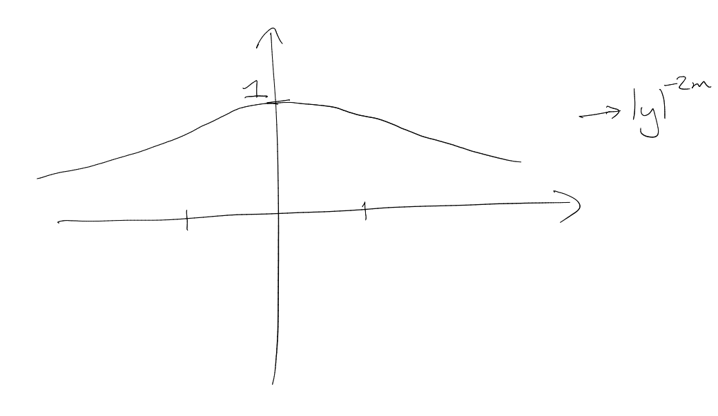
The equality here is the Layer cake formula, which is true for any
.
Let . Study the
random variable .
Fact:
(to
check, use the Taylor series). So we can get
By symmetry,
Choose
:
Use in
Layer cake:
Lower bound: use
Hölder’s inequality.
.
.
□
Can you find a more intuitive proof? E-mail Dominique Maldague.
Corollary.
.
Useful for exercises!
Return to Fourier restriction context.
Both are
-periodic. So
study them on .
,
for
.
,
for
.
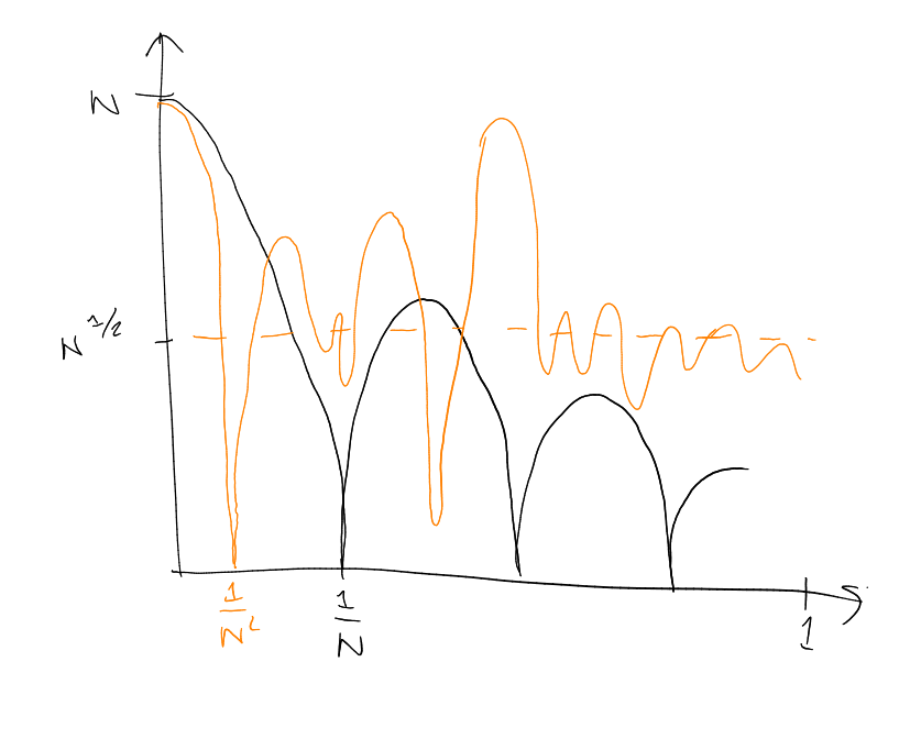
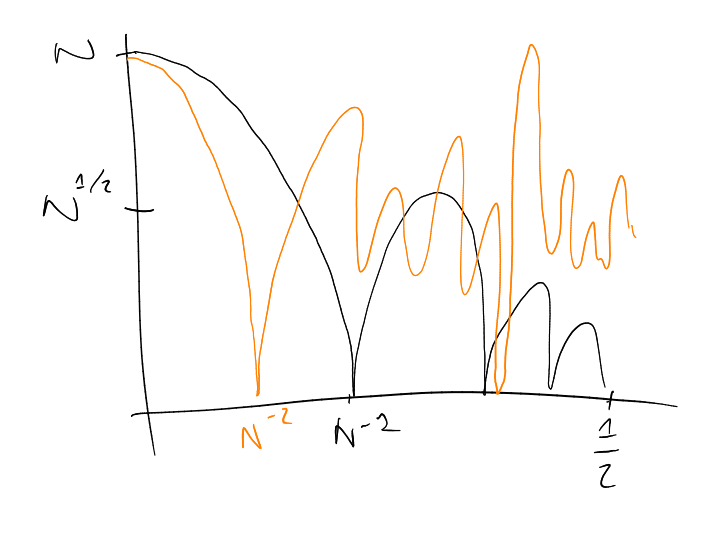
For the first one,
(organised behaviour)
dominates as soon as ,
and for the second one,
dominates for
(“square root cancellation behaviour lasts for longer”).
2 Exponential sums in
Recall: studying . When
does not have (linear) structure,
expect (“sqrt cancellation”)
in an appropriate sense (in ),
more than when
is structured.
Linear
vs
convex
.
Have
Have
on
, and
on
.
does not
distinguish .
does not distinguish.
However,
does.
What about ?
We don’t usually study this range because the estimates tend to be trivial / not interesting.
Focus on .
Preduct size of
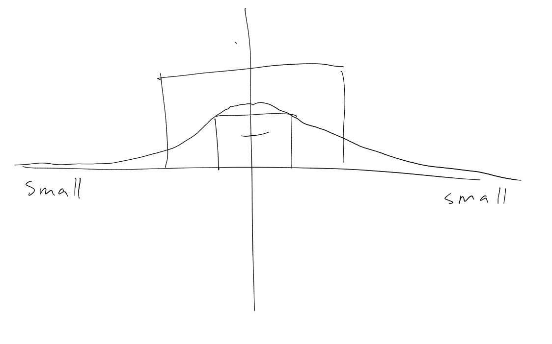
Square root cancellation lower bound:
.
Constant integral lower bound:
,
.
Note that for the
bound, is
bigger than
(as long as ),
so the constant integral dominates!
For , if
, the square root cancellation
dominates, but for
the constant integral takes over.
Assuming:
Theorem 2.1.
-
- Then:
Proof.
Consider: ,
.
Note that this is sharp when .
. Focus
on .
The integral
vanishes unless .
Number Theory lemma: If ,
then
Follows
from unique prime factorisation.
Warning.
The above lemma is false.
See correction later.
For fixed ,
Hence
We will now use
to mean up to
powers of .
:
,
,
,
.
:
Assuming:
Theorem 2.2.
-
Then:
Sharp by .
Positive take away: estimates are sharp, proofs are elementary. Easy to think of sharp examples.
Number Theory counting idea shows:
Sharp, .
Strichartz estimate for periodic Schrödinger equation, observed by Bourgain in 1990s.
Negatives: on
, but this technique can only
work on even integer values of .
,
only
sharp Strichartz estimates per Schrödinger until 2015!
2015: Bourgain-Demeter proved
sharp decoupling estimate. Gives sharp Strichartz estimate for Schrödinger in
for all
.
Proved earlier:
(where
means
).
Conjecture:
,
,
.
Example: .
3 Introduction to Fourier Transform
Correction for lecture 2: Number Theory Lemma.
True statements:
and
.
See Terence Tao notes online.
Explaining :
,
such
that for
all .
We will be using to
mean “ but up to
sub-polynomial in ”.
Question:
For
example, .
Recall:
means .
,
,
.
Reasonable conjecture?
Yes, reasonable.
Khinchin’s inequality: May select
so that
Constant integral: .
.
Warning.
Enemy scenario:
(technically
if we want to satisfy the conditions mentioned above).
. Length
vector
with
many s.
Have:
We can calculate that the above expression is in fact
(which breaks the
conjecture until ).
It turns out that this is (roughly speaking) the only problem.
Why do we care?
,
. Then
Convex
sequences have minimal additive energy.
Decoupling doesn’t know how to take advantage of
.
3.1 Fourier Transform on
,
Schwartz
function:
for all .
is the spatial
variable, and
is the frequency variable.
Facts:
-
If ,
then .
-
Plancherel’s Theorem: .
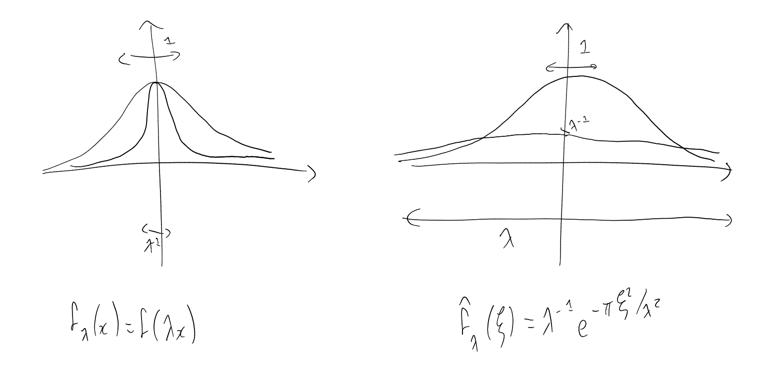
-
,
-
On the left: mass of is
smashed by a factor of . On
the right: the mass of is
stretched by a factor of ,
“ normalized”.
is independent
of .
There is a general formula for
where
is an affine transformation.
-
.
-
Translations are dual to modulations:
Basic question about :
to
boundedness?
Plancherel’s:
(isometry
on ).
,
:
(contraction
from to
).
By interpolation (Marcinkiewicz):
for ,
(Hausdorff-Young inequality).
Are there any other
for which
Attempt 1: Let (compactly
supported smooth function on ),
with .
Consider .
Choose
so that
are not overlapping. Then
Also
We
will use Khinchin’s inequality.
.
4 Introduction to Fourier Restriction
Theorem (Hausdorff-Young inequality).
Assuming that:
Proof.
The inequality is true for ,
and for ,
the inequality is true since we have equality (Plancherel).
For values in between we can interpolate. □
Are there any other
for which
We saw that
was necessary (translations / modulations, Khinchin’s inequality).
Scaling: Plug in
which is -normalised
(). Then
which is
-normalised
().
So we need
for all :
So we
need ,
i.e. .
Classical questions
What is the smallest
constant such that ?
Which functions
satisfy ?
2014:
Fourier restriction
asks which
permit estimates
( is the restricted
frequency set, ).
Example.
(measure
subset of ).
means
Always:
true for
all .
In the second example, only this trivial statement is true (i.e.
is false for all
other values for ).
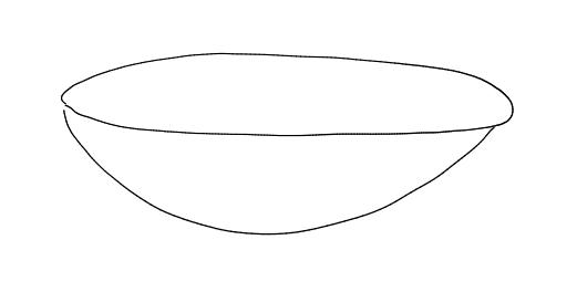
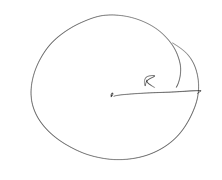
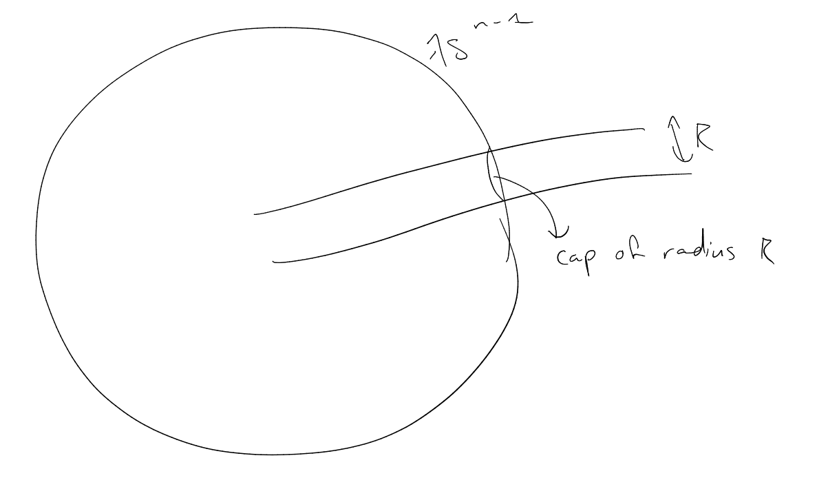
Let be the unit
sphere in .
Consider
where
uses the usual
surface measure
on .
Notation.
We may
call
the
“inverse Fourier transform”.
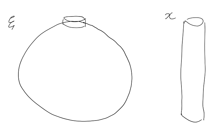
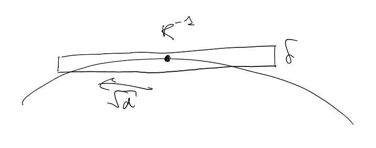
Let ,
-valued,
on
, with
support in .
May also assume
is -valued,
on
.
bounded,
.
behaves
like in
.
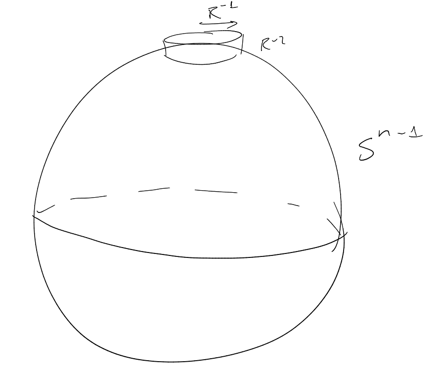
Consider dilates ,
.
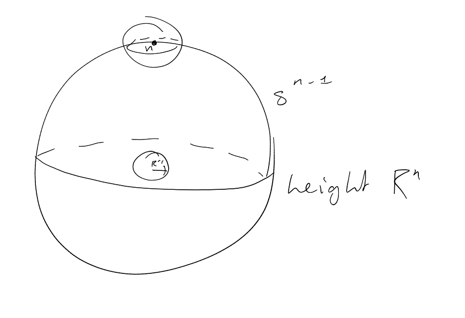
Frequency side
(-norm).
cap of
radius .
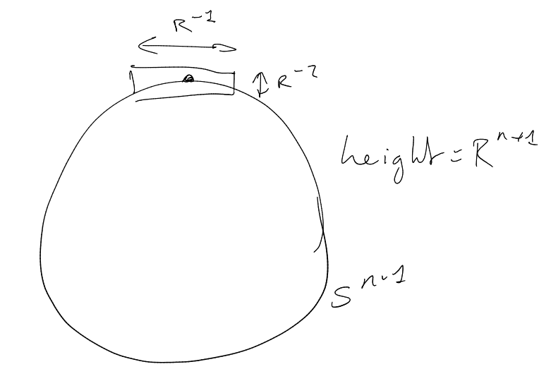
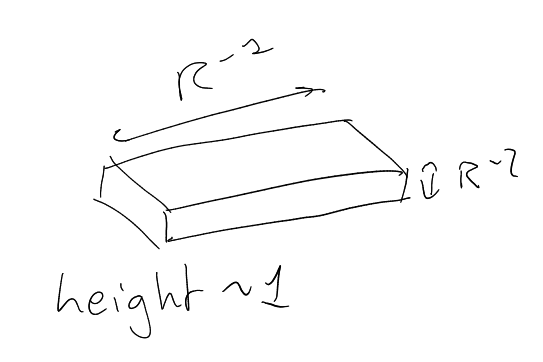
Spacial side
(in -norm).
height ,
.
,
.
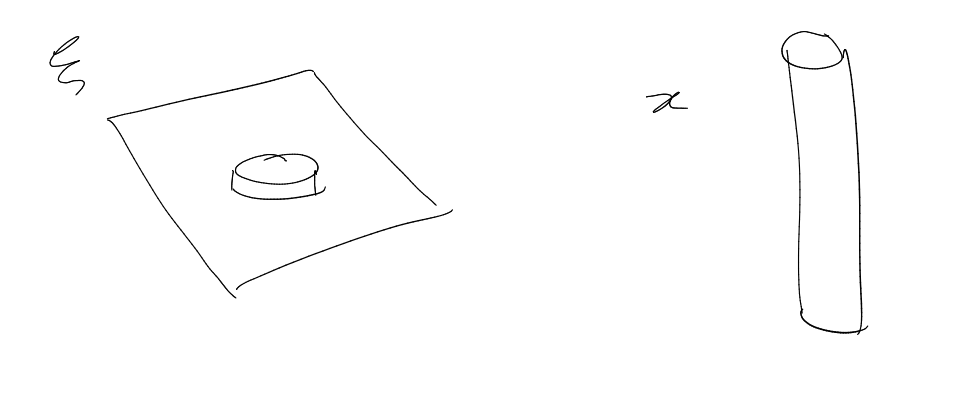
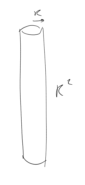
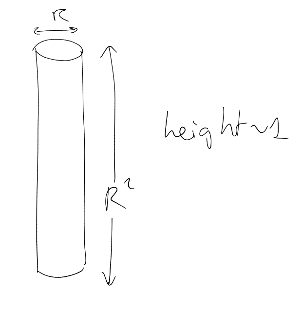
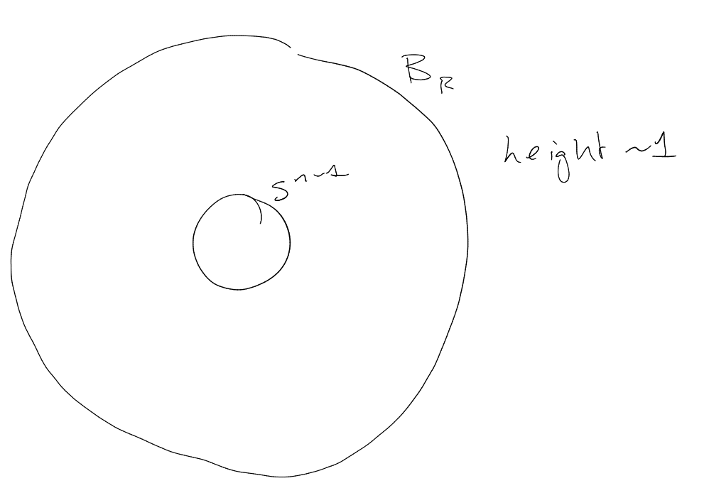
Consider: .
Frequency: .
.
Spatial side:
(-norm).
.
,
. Implies
B.
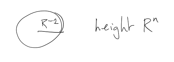
On Monday, we will build examples
such that
sees all of .
.
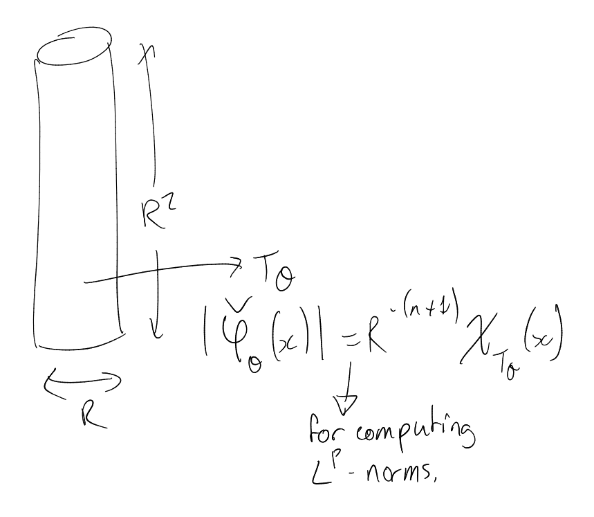
Consider the statement
(recall that we
called this ).
Fix ,
. For
computing
norms, .
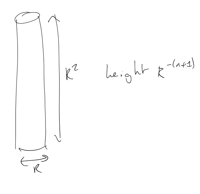
Wave packet function with localised spatial and frequency behaviour.
Last time: .
Frequency:
Spatial:
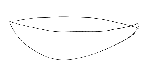
Note: sphere near
looks like ,
.
Naive attempt:
Frequency:
Spatial:
.
Deduce: , so
(trivial).
on
made
easy to
compute.
Could we improve things?
Could think about :
then ,
. This is
more efficient, but we can’t take a limit. So not so useful.
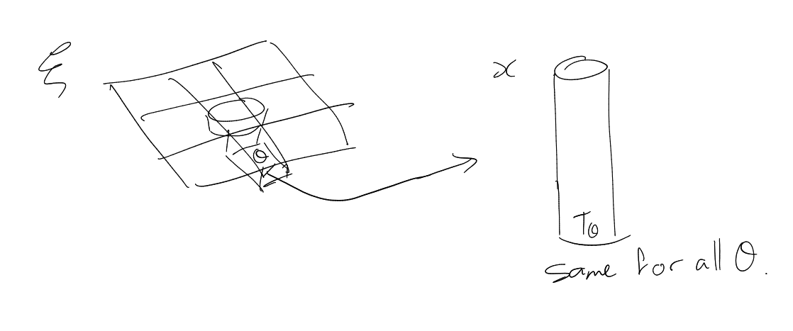
Build a function
which satisfies
on .
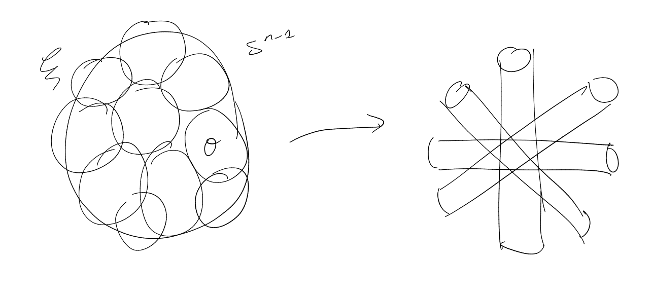
Let be a maximal
collection of -spaced
points on
().
For each ,
let be
an affine map which sends
Define
,
.
on
(actually on
-neighbourhood
of ).
.
.
Frequency:
Spatial:
.
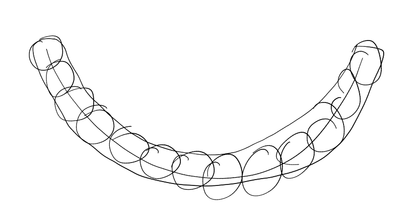
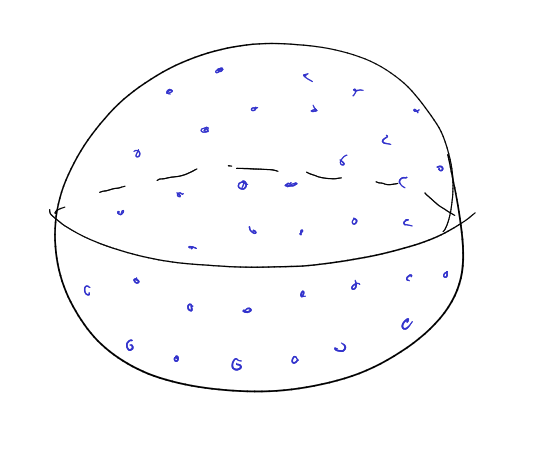
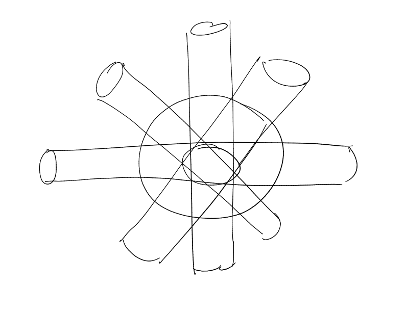
“bush of tubes”
many
tubes in
-separated
directions
Compute
 (Rn−1)
p
2 ⋅Rn +
(Rn−1)
p
2 ⋅Rn +  (∗)
(∗)
Consider overlap of
on
().
Average overlap on :
Not too hard to check that the number of active
on is
.
Now calculate:
Two cases: either
dominates or the other
term dominates. So .
5 Equivalent Versions of Fourier Restriction
Searching for
for which
Reminder:
means
Conjecture (Restriction Conjecture).
if and only if
and .
First proved for
by Fefferman (1970) and Zygmund (1974).
Special things happen in ,
classical harmonic analysis techniques apply.
Same conjecture for ,
where
.
For ,
open and active!
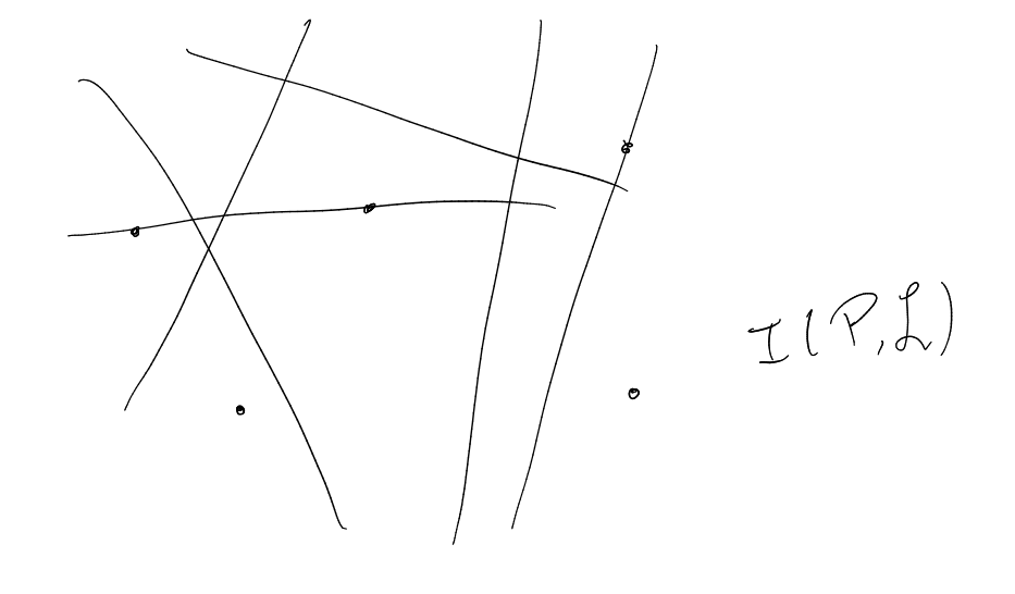
Restriction theory can be used to deduce continuum incidence geometry estimates.
Surprisingly, we can go the other way too (very recent progress, whereas the above direction has been well-known since
at least the s).
Equivalent formulations of
Dual version is called “Fourier extension”:
(). The
integral equals:
Call the last inequality .
Local, dual version: allows us to work with functions, F.T.
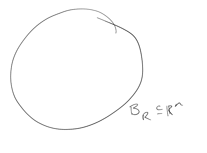
For any ,
any , we
have
for all
with
.
Call this .
. First thing bounds
, while secound
thing bounds
when we have .
Let ,
. Try to
express
in trems of ext. op.
 (∗)
using RPn−1∗(q′→ p′)
Goal is to bound this last expression by Lucy
case: ,
i.e. .
Then
(actually
since
approximately
constant on )
(∗)
using RPn−1∗(q′→ p′)
Goal is to bound this last expression by Lucy
case: ,
i.e. .
Then
(actually
since
approximately
constant on )
continued.
Spatial:
Frequency :
,
,
Aiming for
Lucky case: .
()
Unlucky case: .
Hölder’s inequality goes in the wrong direction:
for all
,
.
This is equality if
is constant on .
PAUSE THIS.
Useful Harmonic Analysis tool
The locally constant property.
Convolution: Let .
Define
by
See
Young’s convolution: when
.
Example.
(
is the unit ball in ),
RHS is “average
value of
on
”.
“ is approximately constant
on balls of radius ”.
Support property: ,
,
.
Convolution and Fourier Transform: .
Locally constant property: Let ,
. Then for any
unit ball
and any ,
is
on
.
Digesting .
For any unit interval ,
,
Suppose this:
LHS has to be constant.
Lemma (Locally constant property).
Assuming that:
-
-
Then for any unit ball
and any
,
The proof of this fact is more important than the statement – we will be using the strategy in
future.
Proof of locally constant property.
Let ,
.
Let
such that
on ,
.
By Fourier inversion:
Let
(unit
ball in
).
Returning to
where
satisfies
on
,
.
supported in
-neighbourhood
of .
Repeat steps of proof:
6 Tube incidence implications of Fourier restriction
Last time: LOCALLY CONSTANT PROPERTY (think of it more as “heuristic”).
If
then
-
(1)
Imagine
on unit balls.
-
(2)
.
What if
(so on
-balls)?
where
.
is approximately
averaging over a -ball.
is approximately
averaging over -balls.
What about ?
Same thing happens, because will have
Fourier support in , and taking absolute
values means we don’t notice the
(modulation).
Returning to .
,
on
,
.
Last lecture
Can choose
such that
-
.
-
.
Case 1: .
LHS of
(using Hölder) is
 ∼1
(Holder)
≲|IR−1|1−p′
q′ (∫
ℝn ∫
ℝn|f^|q′
(ξ − η)|φBR^|(η)dηdξ)
p′
q′
∼|IR−1|1−p′
q′ (∫
ℝn|f^|q′(ξ)dξ)
p′
q′
∼1
(Holder)
≲|IR−1|1−p′
q′ (∫
ℝn ∫
ℝn|f^|q′
(ξ − η)|φBR^|(η)dηdξ)
p′
q′
∼|IR−1|1−p′
q′ (∫
ℝn|f^|q′(ξ)dξ)
p′
q′
Case 2: .
Use for
intuition.
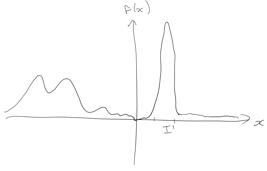
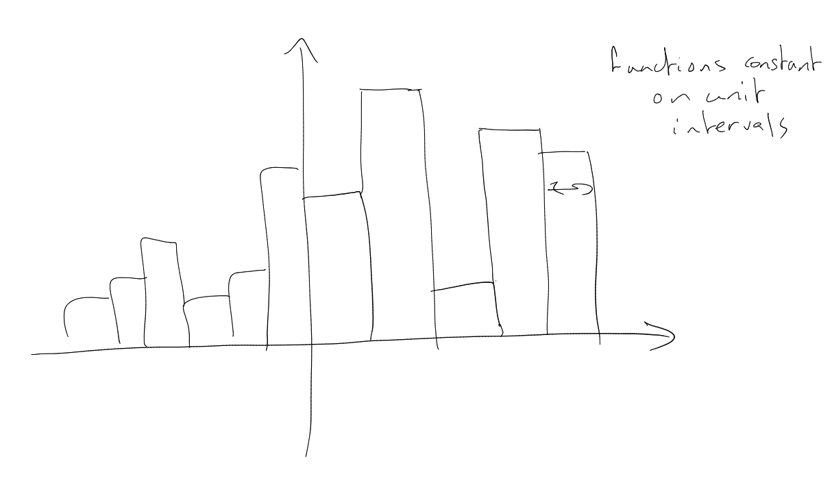
Imagine a function which is
approximately constant on each
cube .
Think of as
.
Note
Therefore, if
.
( for all
).
for
.
Important: locally constant property means we didn’t need
, like
before.
Make the intuition rigorous.
Consider the integral:
˙
Index


![∫ ∑ ∫
|f(x)|2dx = e((n− mx )dx = N).
[0,1] n,m [0,1]](FR10x.svg)
![∫ ∑ ∫
|g(x )|2 = e((n2 − m2 )x)dx = N.
[0,1] n,m [0,1]](FR11x.svg)
![∫
|f(x)|pdx ≥ N p∕2 + N p−1
[0,1]](FR12x.svg)
![∫
|f(x)|pdx ≥ N p∕2+ N p−2.
[0,1]](FR13x.svg)
![∫ ∫
|f(x)|2dx = N = |g(x)|2dx.
[0,1] [0,1]](FR14x.svg)
![∫ p
|f|.
[0,1]](FR15x.svg)
![∫ ( ∫ ) 2p
2 H ölder’s 2⋅p2 □
N = [0,1]|f | ≤ [0,1]|f| (1)](FR16x.svg)

![| |4
∫ ||∑ 2 || ∑ ∑ ∑ ∑ ------∫ 2 2 2 2
[0,1]|| bne(n x)|| dx = bn1bn2bn3bn4 [0,1]e((n1 + n2 − n3 − n4)x)dx.
n n1 n2 n3 n4](FR18x.svg)


![∫
p p− 4 4 CS 12 p−4 4 p2−2 p
[0,1]|h| ≾ ∥h∥∞ ∥bn∥2 ≤ (N ∥bn∥2) ∥bn∥2 ≈ N ∥bn∥2.](FR21x.svg)

![| |
∫ ||∑ ( n2 )||p p p
N −2 2 || e N-2x || dx ≤ (1+ N 2−2)∥bn ∥2.
[0,N ] n∼N](FR23x.svg)
![∫ | |p
− ||∑ b e(a x)|| dx ≲ (1 + N p2−2)∥b ∥p
[0,N2]||n∈N n n || n 2](FR24x.svg)

![∫ || ||p
− ||∑ bne(anx)|| dx ≾ (1 +N p2− 2)∥bn∥2.
[0,N2]|n∼N | 2](FR26x.svg)
![∫ | |p ∫ | |p2
||∑ || ||∑ 2||
− [0,N2]|| bne(anx)|| dx ∼ − [0,N2]|| |bn| || dx.
n n](FR27x.svg)
![∫ ||∑ ||p ∫
− || e(anx)|| dx ≳ -12 N pdx ∼ N p−2 = N p2− 2∥bn∥p2.
[0,N2]|n | N [0,c]](FR28x.svg)
![| |
∫ || ∑ ( ∘ -2- )||p ∫ || ∑ ( ) ||p
− || e m-x || dx = − || e √m--x ||dx
[0,N2]|N≤m2≤2N N | [0,N2]|m2∼N N |](FR29x.svg)
![| |
∫ ||∑ ||4 2 2
− 2|| e(anx )|| dx ≾ N = |{an}| .
[0,N ] n](FR30x.svg)


![∑ ∫ ||∑ ||p2
(∗) ∼ || χT𝜃|| dx.
R<λ<R2 λ<|x|<2λ | 𝜃 |
−(◟n−1)-◝◜2(n−1◞)p n
[λ R ]2λ](FR57x.svg)
![−(n+1)p 2n (n− 1)p n
1 ≲ R [R +R 2R ].](FR58x.svg)