Entropy Methods in Combinatorics - Cambridge III notes

Entropy Methods in Combinatorics
Daniel Naylor

1The Khinchin (Shannon?) axioms for entropy
2A special case of Sidorenko’s conjecture
3Brégman’s Theorem
4Shearer’s lemma and applications
5The union-closed conjecture
6Entropy in additive combinatorics
7A proof of Marton’s conjecture in

𝔽_{2}^{n}

Index

1 The Khinchin (Shannon?) axioms for entropy

Note. In this course, “random variable” will mean “discrete random variable” (unless otherwise specified).

All logarithms will be base $2$ (unless otherwise specified).

Definition (Entropy). The entropy of a discrete random variable $X$ is a quantity $H [X]$ that takes real values and has the following properties:

(i) Normalisation: If $X$ is uniform on ${0, 1}$ then $H [X] = 1$ .
(ii) Invariance: If $X$ takes values in $A$ , $Y$ takes values in $B$ , $f$ is a bijection from $A$ to $B$ , and for every $a \in A$ we have $ℙ [X = a] = ℙ [Y = f (a)]$ , then $H [Y] = H [X]$ .
(iii) Extendability: If $X$ takes values in a set $A$ , and $B$ is disjoint from $A$ , $Y$ takes values in $A \cup B$ , and for all $a \in A$ we have $ℙ [Y = a] = ℙ [X = a]$ , then $H [Y] = H [X]$ .
(iv) Maximality: If $X$ takes values in a finite set $A$ and $Y$ is uniformly distributed in $A$ , then $H [X] \leq H [Y]$ .
(v) Continuity: $H$ depends continuously on $X$ with respect to total variation distance (defined by the distance between $X$ and $Y$ is $\sup_{E} | ℙ [X \in E] - ℙ [Y \in E] |$ ).

For the last axiom we need a definition:

Let $X$ and $Y$ be random variables. The conditional entropy $H [X | Y]$ of $X$ given $Y$ is

\sum_{y} ℙ [Y = y] H [X | Y = y] .

(vi) Additivity: $H [X, Y] = H [Y] + H [X | Y]$ .

Lemma 1.1. Assuming that:

$X$ and $Y$ are independent random variables

Then

H [X, Y] = H [X] + H [Y] .

Proof. $H [X | Y] = \sum_{y} ℙ [Y = y] H [X | Y = y]$ .

Since $X$ and $Y$ are independent, the distribution of $X$ is unaffected by knowing $Y$ (so by invariance, $H [X | Y = y] = H [X]$ ), so

H [X | Y = y] = H [X]

for all $y$ , which gives the result. □

Corollary 1.2. If $X_{1}, \dots, X_{n}$ are independent, then

H [X_{1}, \dots, X_{n}] = H [X_{1}] + \dots + H [X_{n}] .

Proof. Lemma 1.1 and obvious induction. □

Lemma 1.3 (Chain rule). Assuming that:

$X_{1}, \dots, X_{n}$ are random variables

Then

H [X_{1}, \dots, X_{n}] = H [X_{1}] + H [X_{2} | X_{1}] + H [X_{3} | X_{1}, X_{2}] + \dots + H [X_{n} | X_{1}, \dots, X_{n - 1}] .

Proof. The case $n = 2$ is additivity. In general,

H [X_{1}, \dots, X_{n}] = H [X_{1}, \dots, X_{n - 1}] + H [X_{n} | X_{1}, \dots, X_{n - 1}]

so we are done by induction. □

Lemma 1.4. Assuming that:

$Y = f (X)$

Then

H [X, Y] = H [X] .

Also,

H [Z | X, Y] = H [Z | X] .

Proof. The map $g : x \mapsto (x, f (x))$ is a bijection, and $(X, Y) = g (X)$ . So the first statement follows by invariance. For the second statement:

\begin{array}{l} H [Z | X, Y] & = H [Z, X, Y] - H [X, Y] & (by additivity) \\ = H [Z, X] - H [X] & (by first part) \\ = H [Z | X] & (by additivity) □ \end{array}

Lemma 1.5. Assuming that:

$X$ takes only one value

Then

H [X] = 0

Proof. $X$ and $X$ are independent. Therefore, by Lemma 1.1, $H [X, X] = 2 H [X]$ . But by invariance, $H [X, X] = H [X]$ . So $H [X] = 0$ . □

Proposition 1.6. Assuming that:

$X$ is uniformly distributed on a set of size $2^{n}$

Then

H [X] = n

Proof. Let $X_{1}, \dots, X_{n}$ be independent random variables uniformly distributed on ${0, 1}$ . By Corollary 1.2 and normalisation, $H [X_{1}, \dots, X_{n}] = n$ . But $(X_{1}, \dots, X_{n})$ is uniformly distributed on ${0, 1}^{n}$ , so by invariance, the result follows. □

Proposition 1.7. Assuming that:

$X$ is uniformly distributed on a set $A$ of size $n$

Then

H [X] = \log n

Reminder: $\log$ here is to the base $2$ (which is the convention for this course).

Proof. Let $r$ be a positive integer and let $X_{1}, \dots, X_{r}$ be independent copies of $X$ .

Then $(X_{1}, \dots, X_{r})$ is uniform on $A^{r}$ and

H [X_{1}, \dots, X_{r}] = r H [X] .

Now pick $k$ such that $2^{k} \leq n^{r} \leq 2^{k + 1}$ . Then by invariance, maximality, and Proposition 1.6, we have that

k \leq r H [X] \leq k + 1 .

\frac{k}{r} \leq \log n \leq \frac{k + 1}{r} ⟹ \frac{k}{r} \leq H [X] \leq \frac{k + 1}{r} \forall k, r

Therefore, $H [X] = \log n$ as claimed. □

Notation. We will write $p_{a} = ℙ [X = a]$ .

We will also use the notation $[n] = {1, 2, \dots, n}$ .

Theorem 1.8 (Khinchin). Assuming that:

$H$ satisfies the Khinchin axioms
$X$ takes values in a finite set $A$

Then

H [X] = \sum_{a \in A} p_{a} \log (\frac{1}{p_{a}}) .

Proof. First we do the case where all $p_{a}$ are rational (and then can finish easily by the continuity axiom).

Pick $n \in ℕ$ such that for all $a$ , there is some $m_{a} \in ℕ \cup {0}$ such that $p_{a} = \frac{m_{a}}{n}$ .

Let $Z$ be uniform on $[n]$ . Let $(E_{a} : a \in A)$ be a partition of $[n]$ into sets with $| E_{a} | = m_{a}$ . By invariance we may assume that $X = a ⟺ Z \in E_{a}$ . Then

\begin{array}{l} \log n & = H [Z] \\ = H [Z, X] \\ = H [X] + H [Z | X] \\ = H [X] + \sum_{a \in A} p_{a} H [Z | X = a] \\ = H [X] + \sum_{a \in A} p_{a} \log (m_{a}) \\ = H [X] + \sum_{a \in A} p_{a} (\log p_{a} + \log n) \end{array}

Hence

H [X] = - \sum_{a \in A} p_{a} \log p_{a} = \sum_{a \in A} p_{a} \log (\frac{1}{p_{a}}) .

By continuity, since this holds if all $p_{a}$ are rational, we conclude that the formula holds in general. □

Corollary 1.9. Assuming that:

$X$ and $Y$ random variables

Then

H [X] \geq 0

and

H [X | Y] \geq 0

Proof. Immediate consequence of Theorem 1.8. □

Corollary 1.10. Assuming that:

$Y = f (X)$

Then

H [Y] \leq H [X]

Proof. $H [X] = H [X, Y] = H [Y] + H [X | Y]$ . But $H [X | Y] \geq 0$ . □

Proposition 1.11 (Subadditivity). Assuming that:

$X$ and $Y$ be random variables

Then

H [X, Y] \leq H [X] + H [Y]

Proof. Note that for any two random variables $X, Y$ we have

\begin{array}{l} H [X, Y] & \leq H [X] + H [Y] \\ ⟺ H [X | Y] & \leq H [X] \\ ⟺ H [Y | X] & \leq H [Y] \end{array}

Next, observe that $H [X | Y] \leq H [X]$ if $X$ is uniform on a finite set. That is because

\begin{array}{l} H [X | Y] & = \sum_{y} ℙ [Y = y] H [X | Y = y] \\ \leq \sum_{y} ℙ [Y = y] H [X] & (by maximality) \\ = H [X] \end{array}

By the equivalence noted above, we also have that $H [X | Y] \leq H [X]$ if $Y$ is uniform.

Now let $p_{a b} = ℙ [(X, Y) = (a, b)]$ and assume that all $p_{a b}$ are rational. Pick $n$ such that we can write $p_{a b} = \frac{m_{a b}}{n}$ with each $m_{a b}$ an integer. Partition $[n]$ into sets $E_{a b}$ of size $m_{a b}$ . Let $Z$ be uniform on $[n]$ . Without loss of generality (by invariance) $(X, Y) = (a, b) ⟺ Z \in E_{a b}$ .

Let $E_{b} = \cup_{a} E_{a b}$ for each $b$ . So $Y = b ⟺ Z \in E_{b}$ . Now define a random variable $W$ as follows: If $Y = b$ , then $W \in E_{b}$ , but then $W$ is uniformly distributed in $E_{b}$ and independent of $X$ (or $Z$ if you prefer).

So $W$ and $X$ are conditionally independent given $Y$ , and $W$ is uniform on $[n]$ .

Then

\begin{array}{l} H [X | Y] & = H [X | Y, W] & (by conditional independence) \\ = H [X | W] & (as W determines Y) \\ \leq H [X] & (as W is uniform) \end{array}

By continuity, we get the result for general probabilities. □

Corollary 1.12. Assuming that:

$X$ a random variable

Then

H [X] \geq 0

Proof (Without using formula). By Subadditivity, $H [X | X] \leq H [X]$ . But $H [X | X] = 0$ . □

Corollary 1.13. Assuming that:

$X_{1}, \dots, X_{n}$ are random variables

Then

H [X_{1}, \dots, X_{n}] \leq H [X_{1}] + \dots + H [X_{n}] .

Proof. Induction using Subadditivity. □

Proposition 1.14 (Submodularity). Assuming that:

$X, Y, Z$ are random variables

Then

H [X | Y, Z] \leq H [X | Z] .

Proof. Calculate:

\begin{array}{l} H [X | Y, Z] & = \sum_{z} ℙ [Z = z] H [X | Y, Z = z] \\ \leq \sum_{z} ℙ [Z = z] H [X | Z = z] \\ = H [X | Z] □ \end{array}

Submodularity can be expressed in many ways.

Expanding using additivity gives the following inequalities:

\begin{array}{l} H [X, Y, Z] - H [Y, Z] & \leq H [X, Z] - H [Z] \\ H [X, Y, Z] & \leq H [X, Z] + H [Y, Z] - H [Z] \\ H [X, Y, Z] + H [Z] & \leq H [X, Z] + H [Y, Z] \end{array}

Lemma 1.15. Assuming that:

$X, Y, Z$ random variables
$Z = f (Y)$

Then

H [X | Y] \leq H [X | Z] .

Proof.

\begin{array}{l} H [X | Y] & = H [X, Y] - H [Y] \\ = H [X, Y, Z] - H [Y, Z] \\ \leq H [X, Z] - H [Z] & (Submodularity) \\ = H [X | Z] & □ \end{array}

Lemma 1.16. Assuming that:

$X, Y, Z$ random variables
$Z = f (X) = g (Y)$

Then

H [X, Y] + H [Z] \leq H [X] + H [Y] .

Proof. Submodularity says:

H [X, Y, Z] = H [Z] \leq H [X, Z] + H [Y, Z]

which implies the result since $Z$ depends on $X$ and $Y$ . □

Lemma 1.17. Assuming that:

$X$ takes values in a finite set $A$
$Y$ is uniform on $A$
$H [X] = H [Y]$

Then

X

is uniform.

Proof. Let $p_{a} = ℙ [X = a]$ . Then

\begin{array}{l} H [X] & = \sum_{a \in A} p_{a} \log (\frac{1}{p_{a}}) \\ = | A | \sum_{a \in A} p_{a} \log (\frac{1}{p_{a}}) \end{array}

The function $x \mapsto x \log \frac{1}{x}$ is concave on $[0, 1]$ . So, by Jensen’s inequality this is at most

| A | (𝔼_{a} p_{a}) \log (\frac{1}{𝔼_{a} p_{a}}) = \log (| A |) = H [Y] .

Equality holds if and only if $a \mapsto p_{a}$ is constant – i.e. $X$ is uniform. □

Corollary 1.18. Assuming that:

$X, Y$ random variables
$H [X, Y] = H [X] + H [Y]$

Then

X

and

Y

are independent.

Proof. We go through the proof of Subadditivity and check when equality holds.

Suppose that $X$ is uniform on $A$ . Then

\begin{array}{l} H [X | Y] & = \sum_{y} ℙ [Y = y] H [X | Y = y] \\ \leq H [X] \end{array}

with equality if and only if $H [X | Y = y]$ is uniform on $A$ for all $y$ (by Lemma 1.17), which implies that $X$ and $Y$ are independent.

At the last stage of the proof we used

H [X | Y] = H [X | Y, W] = H [X | W] \leq H [X]

where $W$ was uniform. So equality holds only if $X$ and $W$ are independent, which implies (since $Y$ depends on $W$ ) that $X$ and $Y$ are indpendent. □

Definition (Mutual information). Let $X$ and $Y$ be random variables. The mutual information $I [X : Y]$ is

\begin{array}{l} H [X] + H [Y] - H [X, Y] & = H [X] - H [X | Y] \\ = H [Y] - H [Y | X] \end{array}

Subadditivity is equivalent to the statement that $I [X : Y] \geq 0$ and Corollary 1.18 implies that $I [X : Y] = 0$ if and only if $X$ and $Y$ are independent.

Note that

H [X, Y] = H [X] + H [Y] - I [X : Y] .

Definition (Conditional mutual information). Let $X$ , $Y$ and $Z$ be random variables. The conditional mutual information of $X$ and $Y$ given $Z$ , denoted by $I [X : Y | Z]$ is

\begin{array}{l} \sum_{z} ℙ [Z = z] I [X | Z = z : Y | Z = z] \\ = \sum_{z} ℙ [Z = z] (H [X | Z = z] + H [Y | Z = z] - H [X, Y | Z = z]) \\ = H [X | Z] + H [Y | Z] - H [X, Y | Z] \\ = H [X, Z] + H [Y, Z] - H [X, Y, Z] - H [Z] \end{array}

Submodularity is equivalent to the statement that $I [X : Y | Z] \geq 0$ .

2 A special case of Sidorenko’s conjecture

Let $G$ be a bipartite graph with vertex sets $X$ and $Y$ (finite) and density $α$ (defined to be $\frac{| E (G) |}{| X | | Y |}$ ). Let $H$ be another (think of it as ‘small’) bipartite graph with vertex sets $U$ and $V$ and $m$ edges.

Now let $ϕ : U \to X$ and $ψ : V \to Y$ be random functions. Say that $(ϕ, ψ)$ is a homomorphism if $ϕ (x) ϕ (y) \in E (G)$ for every $x y \in E (H)$ .

Sidorenko conjectured that: for every $G, H$ , we have

ℙ [(ϕ, ψ) is a homomorphism] \geq α^{m} .

Not hard to prove when $H$ is $K_{r, s}$ . Also not hard to prove when $H$ is $K_{2, 2}$ (use Cauchy Schwarz).

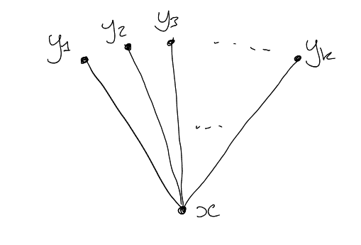
Theorem 2.1. Sidorenko’s conjecture is true if $H$ is a path of length $3$ .

Proof. We want to show that if $G$ is a bipartite graph of density $α$ with vertex sets $X, Y$ of size $m$ and $n$ and we choose $x_{1}, x_{2} \in X$ , $y_{1}, y_{2} \in Y$ independently at random, then

ℙ [x_{1} y_{1}, x_{2} y_{2}, x_{3} y_{3} \in E (G)] \geq α^{3} .

It would be enough to let $P$ be a P3 chosen uniformly at random and show that $H [P] \geq \log (α^{3} m^{2} n^{2})$ .

Instead we shall define a different random variable taking values in the set of all P3s (and then apply maximality).

To do this, let $(X_{1}, Y_{1})$ be a random edge of $G$ (with $X_{1}, \in X$ , $Y_{1} \in Y$ ). Now let $X_{2}$ be a random neighbour of $Y_{1}$ and let $Y_{2}$ be a random neighbour of $X_{2}$ .

It will be enough to prove that

H [X_{1}, Y_{1}, X_{2}, Y_{2}] \geq \log (α^{3} m^{2} n^{2}) .

We can choose $X_{1} Y_{1}$ in three equivalent ways:

(1) Pick an edge uniformly from all edges.
(2) Pick a vertex $x$ with probability proportional to its degree $d (x)$ , and then pick a random neighbour $y$ of $x$ .
(3) Same with $x$ and $y$ exchanged.

It follows that $Y_{1} = y$ with probability $\frac{d (y)}{| E (G) |}$ , so $X_{2} Y_{1}$ is uniform in $E (G)$ , so $X_{2} = x^{'}$ with probability $\frac{d (x^{'})}{| E (G) |}$ , so $X_{2} Y_{2}$ is uniform in $E (G)$ .

Therefore,

\begin{array}{l} H [X_{1}, Y_{1}, X_{2}, Y_{2}] & = H [X_{1}] + H [Y_{1} | X_{1}] + H [X_{2} | X_{1}, Y_{1}] + H [Y_{2} | X_{1}, Y_{1}, X_{2}] \\ = H [X_{1}] + H [Y_{1} | X_{1}] + H [X_{2} | Y_{1}] + H [Y_{2} | X_{2}] \\ = H [X_{1}] + H [X_{1}, Y_{1}] - H [X_{1}] + H [X_{2}, Y_{1}] - H [Y_{1}] + H [Y_{2}, X_{2}] - H [X_{2}] \\ = 3 H [U_{E (G)}] - H [Y_{1}] - H [X_{2}] \\ \geq 3 H [U_{E (G)}] - H [U_{Y}] - H [U_{X}] \\ = 3 \log (α m n) - \log m - \log n \\ = \log (α^{3} m^{2} n^{2}) \end{array}

So we are done my maximality.

Alternative finish (to avoid using $\log$ !):

Let $X^{'}, Y^{'}$ be uniform in $X, Y$ and independent of each other and $X_{1}, Y_{1}, X_{2}, Y_{2}$ . Then:

\begin{array}{l} H [X_{1}, Y_{2}, X_{2}, Y_{2}, X^{'}, Y^{'}] & = H [X_{1}, Y_{1}, X_{2}, Y_{2}] + H [U_{X}] + H [U_{Y}] \\ \geq 3 H [U_{E (G)}] \end{array}

So by maximality,

# P_{3} s \times | X | \times | Y | \geq | E (G) |^{3} . □

3 Brégman’s Theorem

Definition (Permanent of a matrix). Let $A$ be an $n \times n$ matrix over $ℝ$ . The permanent of $A$ , denoted $per (A)$ , is

\sum_{σ \in S_{n}} \prod_{i = 1}^{n} A_{i σ (i)},

i.e. “the determinant without the signs”.

Let $G$ be a bipartite graph with vertex sets $X, Y$ of size $n$ . Given $(x, y) \in X_{Y}$ , let

A_{x y} = {\begin{matrix} 1 & x y \in E (G) \\ 0 & x y \notin E (G) \end{matrix}

ie $A$ is the bipartite adjacency matrix of $G$ .

Then $per (A)$ is the number of perfect matchings in $G$ .

Brégman’s theorem concerns how large $per (A)$ can be if $A$ is a $01$ -matrix and the sum of entres in the $i$ -th row is $d_{i}$ .

Let $G$ be a disjoint union of $K_{a_{i} a_{i}}$ s for $i = 1, \dots, k$ , with $a_{1} + \dots + a_{k} = n$ .

Then the number of perfect matchings in $G$ is

\prod_{i = 1}^{k} a_{i}! .

Theorem 3.1 (Bregman). Assuming that:

$G$ a bipartite graph with vertex sets $X, Y$ of size $n$

Then the number of perfect matchings in

G

is at most

\prod_{x \in X} {(d (x)!)}^{\frac{1}{d (x)}} .

Proof (Radhakrishnan). Each matching corresponds to a bijection $σ : X \to Y$ such that $x σ (x) \in E (G)$ for every $x$ . Let $σ$ be chosen uniformly from all such bijections.

H [σ] = H [σ (x_{1})] + H [σ (x_{2}) | σ (x_{1})] + \dots + H [σ (x_{n}) | σ (x_{1}), \dots, σ (x_{n - 1})],

where $x_{1}, \dots, x_{n}$ is some enumeration of $X$ .

Then

\begin{array}{l} H [σ (x_{1})] & \leq \log d (x_{1}) \\ H [σ (x_{2}) | σ (x_{1})] & \leq 𝔼_{σ} \log d_{x_{1}}^{σ} (x_{2}) \end{array}

where

d_{x_{i}}^{σ} (x_{2}) = | N (x_{2}) ∖ {σ (x_{1})} | .

In general,

H [σ (x_{i})] σ (x_{1}), \dots, σ (x_{i - 1}) \leq 𝔼_{σ} \log d_{x_{1}, \dots, x_{i - 1}}^{σ} (x_{i}),

where

d_{x_{1}, \dots, x_{i - 1}}^{σ} (x_{i}) = | N (x_{i}) ∖ {σ (x_{1}), \dots, σ (x_{i - 1})} | .

Key idea: we now regard $x_{1}, \dots, x_{n}$ as a random enumeration of $X$ and take the average.

For each $x \in X$ , define the contribution of $x$ to be

\log (d_{x_{1}, \dots, x_{i - 1}}^{σ} (x_{i}))

where $x_{i} = x$ (note that this “contribution” is a random variable rather than a constant).

We shall now fix $σ$ . Let the neighbours of $x$ be $y_{1}, \dots, y_{k}$ .

Then one of the $y_{j}$ will be $σ (x)$ , say $y_{h}$ . Note that $d_{x_{1}, \dots, x_{i - 1}}^{σ} (x_{i})$ (given that $x_{i} = x$ ) is

d (x) - | {j : σ^{- 1} (y_{j}) comes earlier than x = σ^{- 1} (y_{h})} | .

All positions of $σ^{- 1} (y_{h})$ are equally likely, so the average contribution of $x$ is

\frac{1}{d (x)} (\log d (x) + \log (d (x) - 1) + \dots + \log 1) = \frac{1}{d (x)} \log (d (x)!) .

By linearity of expectation,

H [σ] \leq \sum_{x \in X} \frac{1}{d (x)} \log (d (x)!),

so the number of matchings is at most

\prod_{x \in X} {(d (x)!)}^{\frac{1}{d (x)}} . □

Definition ( $1$ -factor). Let $G$ be a graph with $2 n$ vertices. A $1$ -factor in $G$ is a collection of $n$ disjoint edges.

Theorem 3.2 (Kahn-Lovasz). Assuming that:

$G$ a graph with $2 n$ vertices

Then the number of

1

-factors in

G

is at most

\prod_{x \in V (G)} {(d (x)!)}^{\frac{1}{2 d (x)}} .

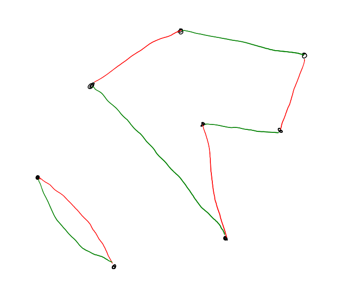
Proof (Alon, Friedman). Let $M$ be the set of $1$ -factors of $G$ , and let $(M_{1}, M_{2})$ be a uniform random element of $M^{2}$ . For each $M_{1}, M_{2}$ , the union $M_{1} \cup M_{2}$ is a collection of disjoint edges and even cycles that covers all the vertices of $G$ .

Call such a union a cover of $G$ by edges and even cycles.

If we are given such a cover, then the number of pairs $(M_{1}, M_{2})$ that could give rise to it is $2^{k}$ , where $k$ is the number of even cycles.

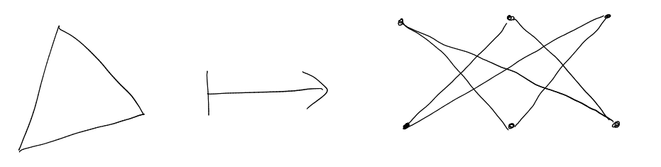
Now let’s build a bipartite graph $G_{2}$ out of $G$ . $G_{2}$ has two vertex sets (call them $V_{1}, V_{2}$ ), both copies of $V (G)$ . Join $x \in V_{1}$ to $y \in V_{2}$ if and only if $x y \in E (G)$ .

For example:

By Bregman, the number of perfect matchings in $G_{2}$ is $\leq \prod_{x \in V (G)} {(d (x)!)}^{\frac{1}{d (x)}}$ . Each matching gives a permutation $σ$ of $V (G)$ , such that $x σ (x) \in E (G)$ for every $x \in V (G)$ .

Each such $σ$ has a cycle decomposition, and each cycle gives a cycle in $G$ . So $σ$ gives a cover of $V (G)$ by isolated vertices, edges and cycles.

Given such a cover with $k$ cycles, each edge can be directed in two ways, so the number of $σ$ that give rise to is is $2^{k}$ , where $k$ is the number of cycles.

So there is an injection from $M^{2}$ to the set of matchings of $G_{2}$ , since every cover by edges and even cycles is a cover by vertices, edges and cycles.

| M |^{2} \leq \prod_{x \in V (G)} {(d (x)!)}^{\frac{1}{d (x)}} . □

4 Shearer’s lemma and applications

Notation. Given a random variable $X = (X_{1}, \dots, X_{n})$ and $A = {a_{1}, \dots, a_{k}} \subset [n]$ with $a_{1} < a_{2} < \dots < a_{k}$ , write $X_{A}$ for the random variable $(X_{a_{1}}, X_{a_{2}}, \dots, X_{a_{k}})$ .

Lemma 4.1 (Shearer). Assuming that:

$X = (X_{1}, \dots, X_{n})$ a random variable
$A$ a family of subsets of $[n]$ such that every $i \in [n]$ belongs to at least $r$ of the sets $A \in A$

Then

H [X_{1}, \dots, X_{n}] \leq \frac{1}{r} \sum_{A \in A} H [X_{A}] .

Proof. For each $a \in [n]$ , write $X_{< a}$ for $(X_{1}, \dots, X_{a - 1})$ .

For each $A \in A$ , $A = {a_{1}, \dots, a_{k}}$ with $a_{1} < \dots < a_{k}$ , we have

\begin{array}{l} H [X_{A}] & = H [X_{a_{1}}] + H [X_{a_{2}} | X_{a_{1}}] + \dots + H [X_{a_{k}} | X_{a_{1}}, \dots, X_{a_{k}}] \\ \geq H [X_{a_{1}} | X_{< a_{1}}] + H [X_{a_{2}} | X_{< a_{2}}] + \dots + H [X_{a_{k}} | X_{< a_{k}}] & (Lemma 1.15) \\ = \sum_{a \in A} H [X_{a} | X_{< a}] \end{array}

Therefore,

\begin{array}{l} \sum_{A \in A} H [X_{A}] & \geq \sum_{A \in A} \sum_{a \in A} H [X_{a} | X_{< a}] \\ \geq r \sum_{a = 1}^{n} H [X_{a} | X_{< a}] \\ = r H [X] □ \end{array}

Alternative version:

Lemma 4.2 (Shearer, expectation version). Assuming that:

$X = (X_{1}, \dots, X_{n})$ a random variable
$A \subset [n]$ a randomly chosen subset of $[n]$ , according to some probability distribution (don’t need any independence conditions!)
for each $i \in [n]$ , $ℙ [i \in A] \geq μ$

Then

H [X] \leq μ^{- 1} 𝔼_{A} H [X_{A}] .

Proof. As before,

H [X_{A}] \geq \sum_{a \in A} H [X_{a} | X_{< a}] .

\begin{array}{l} 𝔼_{A} H [X_{A}] & \geq 𝔼_{A} \sum_{a \in A} H [X_{a} | X_{< a}] \\ \geq μ \sum_{a = 1}^{n} H [X_{a} | X_{< a}] \\ = μ H [X] □ \end{array}

Definition ( $P_{A}$ ). Let $E \subset ℤ^{n}$ and let $A \subset [n]$ . Then we write $P_{A} E$ for the set of all $u \in ℤ^{A}$ such that there exists $v \in ℤ^{[n] ∖ A}$ such that $[u, v] \in E$ , where $[u, v]$ is $u$ suitably intertwined with $v$ (i.e. $u \cup v$ as functions).

Corollary 4.3. Assuming that:

$E \subset ℤ^{n}$
$A$ a family of subsets of $[n]$ such that every $i \in [n]$ is contained at least $r$ sets $A \in A$

Then

| E | \leq \prod_{A \in A} | P_{A} E |^{\frac{1}{r}} .

Proof. Let $X$ be a uniform random element of $E$ . Then by Shearer,

H [X] \leq \frac{1}{r} \sum_{A \in A} H [X_{A}] .

But $X_{A}$ tkaes values in $P_{A} E$ , so

H [X_{A}] \leq \log | P_{A} X,

\log | E | \leq \frac{1}{r} \sum_{A} \log | P_{A} E | . □

If $A = {[n] ∖ {i} : i = 1, \dots, n}$ we get

| E | \leq \prod_{i = 1}^{n} | P_{[n] ∖ {i}} E |^{\frac{1}{n - 1}} .

This case is the discrete Loomis-Whitney theorem.

Theorem 4.4. Assuming that:

$G$ a graph with $m$ edges

Then

G

has at most

\frac{{(2 m)}^{\frac{3}{2}}}{6}

triangles.

Is this bound natural? Yes: if $m = (\binom{n}{2})$ , and we consider a complete graph on $n$ vertices, then we get approximately $\frac{{(2 m)}^{\frac{2}{3}}}{6}$ triangles.

Proof. Let $(X_{1}, X_{2}, X_{3})$ be a random ordered triangle (without loss of generality $G$ has a triangle so that this is possible).

Let $t$ be the number of triangles in $G$ . By Shearer,

\log (6 t) = H [X_{1}, X_{2}, X_{3}] \leq \frac{1}{2} (H [X_{1}, X_{2}] + H [X_{1}, X_{3}] + H [X_{2}, X_{3}]) .

Each edge $H [X_{i}, X_{j}]$ is supported in the set of edges $G$ , given a direction, i.e.

\frac{1}{2} (H [X_{1}, X_{2}] + H [X_{1}, X_{3}] + H [X_{2}, X_{3}]) \leq \frac{3}{2} \cdot \log (2 m) . □

Definition. Let $X$ be a set of size $n$ and let $G$ be a set of graphs with vertex set $X$ . Then $G$ is $Δ$ -intersecting (read as “triangle-intersecting”) if for all $G_{1}, G_{2} \in G$ , $G_{1} \cap G_{2}$ contains a triangle.

Theorem 4.5. Assuming that:

$| V | = n$
$G$ a $Δ$ -intersecting family with vertex set $V$

Then

G

has size at most

2^{(\binom{n}{2}) - 2}

Proof. Let $X$ be chosen uniformly at random from $G$ . We write $V^{(2)}$ for the set of (unordered) pairs of elements of $V$ . Think of any $G \in G$ as a function from $V^{(2)}$ to ${0, 1}$ . So $X = (X_{e} : e \in V^{(2)})$ .

For each $R \subset V$ , let $G_{R}$ be the graph $K_{R} \cup K_{V ∖ R}$

For each $R$ , we shall look at the projection $X_{G_{R}}$ , which we can think of as taking values in the set ${G \cap G_{R} : G \in G} = : G_{R}$ .

Note that if $G_{1}, G_{2} \in G$ , $R \subset [n]$ , then $G_{1} \cap G_{2} \cap G_{R} \neq \emptyset$ , since $G_{1} \cap G_{2}$ contains a triangle, which must intersect $G_{R}$ by Pigeonhole Principle.

Thus, $G_{R}$ is an intersecting family, so it has size at most $2^{| E (G_{R}) | - 1}$ . By Shearer, expectation version,

\begin{array}{l} H [X] & \leq 2 𝔼_{R} H [X_{G_{R}}] & (since each e belongs to G_{R} with probability 1 ∕ 2) \\ \leq 2 𝔼_{R} (| E (G_{R}) | - 1) \\ = 2 (\frac{1}{2} (\binom{m}{2}) - 1) \\ = (\binom{n}{2}) - 2 & □ \end{array}

Definition (Edge-boundary). Let $G$ be a graph and let $A \subset V (G)$ . The edge-boundary $\partial A$ of $A$ is the set of edges $x y$ such that $y \notin A$ .

If $G = ℤ^{n}$ or ${0, 1}^{n}$ and $i \in [n]$ , then the $i$ -th boundary $\partial_{i} A$ is the set of edges $x y \in \partial A$ such that $x - y = \pm e_{i}$ , i.e. $\partial_{i} A$ consists of deges pointing in direction $i$ .

Theorem 4.6 (Edge-isoperimetric inequality in $Z^{n}$ ). Assuming that:

$A \subset ℤ^{n}$ a finite set

Then

| \partial A | \geq 2 n | A |^{\frac{n - 1}{n}}

Proof. By the discrete Loomis-Whitney inequality,

\begin{array}{l} | A | & \leq \prod_{i = 1}^{n} | P_{[n] ∖ {i}} A |^{\frac{1}{n - 1}} \\ = {(\prod_{i = 1}^{n} | P_{[n] ∖ {i}} A |^{\frac{1}{n}})}^{\frac{n}{n - 1}} \\ \leq {(\frac{1}{n} \sum_{i = 1}^{n} | P_{[n] ∖ {i}} A |)}^{\frac{n}{n - 1}} \end{array}

But $| \partial_{i} A | \geq 2 | P_{[n] ∖ {i}} A |$ since each fibre contributes at least 2.

\begin{array}{l} | A | & \leq {(\frac{1}{2 n} \sum_{i = 1}^{n} | \partial_{i} A |)}^{\frac{n}{n - 1}} \\ = {(\frac{1}{2 n} | \partial A |)}^{\frac{n}{n - 1}} □ \end{array}

Theorem 4.7 (Edge-isoperimetric inequality in the cube). Assuming that:

$A \subset {0, 1}^{n}$ (where we take the usual graph)

Then

| \partial A | \geq | A | (n - \log | A |)

Proof. Let $X$ be a uniform random element of $A$ and write $X = (X_{1}, \dots, X_{n})$ . Write $X_{∖ i}$ for $(X_{1}, \dots, X_{i - 1}, X_{i + 1}, \dots, X_{n})$ . By Shearer,

\begin{array}{l} H [X] & \leq \frac{1}{n - 1} \sum_{i = 1}^{r} H [X_{∖ i}] \\ = \frac{1}{n - 1} \sum_{i = 1}^{n} H [X] - H [X_{i} | X_{∖ i}] \end{array}

Hence

\sum_{i = 1}^{n} H [X_{i} | X_{∖ i}] \leq H [X] .

Note

H [X_{i} | X_{∖ i} = u] = {\begin{matrix} 1 & | P_{[n] ∖ {i}}^{- 1} (u) | = 2 \\ 0 & | P_{[n] ∖ {i}}^{- 1} (u) | = 1 \end{matrix}

The number of points of the second kind is $| \partial_{i} A |$ , so $H [X_{i} | X_{∖ i}] = 1 - \frac{| \partial_{i} A |}{| A |}$ . So

\begin{array}{l} H [X] & \geq \sum_{i = 1}^{n} (1 - \frac{| \partial_{i} A |}{| A |}) \\ = n - \frac{| \partial A |}{| A |} \end{array}

Also, $H [X] = \log | A |$ . So we are done. □

Definition (Lower shadow). Let $A$ be a family of sets of size $d$ . The lower shadow $\partial A$ is ${B : | B | = d - 1, \exists A \in A, B \subset A}$ .

Notation. Let $h (x) = x \log \frac{1}{x} + (1 - x) \log \frac{1}{1 - x}$ (for $x \in [0, 1]$ ).

Theorem 4.8 (Kruskal-Katona). Assuming that:

$| A | = (\binom{t}{d}) = \frac{t (t - 1) \dots (t - d - 1)}{d!}$ for some real number $t$

Then

| \partial A | \geq (\binom{t}{d - 1})

Proof. Let $X = (X_{1}, \dots, X_{d})$ be a random ordering of the elements of a uniformly random $A \in A$ . Then

H [X] = \log (d! (\binom{t}{d})) .

Note that $(X_{1}, \dots, X_{d - 1})$ is an ordering of the elements of some $B \in \partial A$ , so

H [X_{1}, \dots, X_{d - 1}] \leq \log ((d - 1)! | \partial A |) .

So it’s enough to show

H [X_{1}, \dots, X_{d - 1}] \geq \log ((d - 1)! (\binom{t}{d - 1})) .

Also,

H [X] = H [X_{1}, \dots, X_{d - 1}] + H [X_{d} | X_{1}, \dots, X_{d - 1}]

and

H [X] = H [X_{1}] + H [X_{2} | X_{1}] + \dots + H [X_{d} | X_{1}, \dots, X_{d - 1}] .

We would like an upper bound for $H [X_{d}] X_{< d}$ . Our strategy will be to obtain a lower bound for $H [X_{k} | X_{< k}]$ in terms of $H [X_{k + 1} | X_{< k + 1}]$ . We shall prove that

2^{H [X_{k} | X_{< k}]} \geq 2^{H [X_{k + 1} | X_{< k + 1}]} + 1 \forall k .

Let $T$ be chosen independently of $X_{1}, \dots, X_{k - 1}$ with

T = {\begin{matrix} 0 & probability p \\ 1 & probability 1 - p \end{matrix}

( $p$ will be chosen and optimised later).

Given $X_{1}, \dots, X_{k - 1}$ , let

X^{*} = {\begin{matrix} X_{k + 1} & T = 0 \\ X_{k} & T = 1 \end{matrix}

Note that $X_{k}$ and $X_{k + 1}$ have the same distribution (given $X_{1}, \dots, X_{k - 1}$ ), so $X^{*}$ does as well. Then

\begin{array}{l} H [X_{k} | X_{< k}] & = H [X^{*} | X_{< k}] \\ \geq H [X^{*} | X_{\leq k}] & (Submodularity) \\ = H [X^{*}, T | X_{\leq k}] & (X_{\leq k} and X^{*} determine T) \\ = H [T | X_{\leq k}] + H [X^{*} | T, X_{\leq k}] & (additivity) \\ = H [T] + p H [X_{k + 1} | X_{1}, \dots, X_{k}] \\ + (1 - p) H [X_{k} | X_{1}, \dots, X_{k}] \\ = h (p) + p s \end{array}

where $h (p) = p \log \frac{1}{p} + (1 - p) \log \frac{1}{1 - p}$ and $s = H [X_{k + 1} | X_{1}, \dots, X_{k}]$ .

It turns out that this is maximised when $p = \frac{2^{s}}{2^{s} + 1}$ . Then we get

\frac{2^{s}}{2^{s} + 1} (\log (2^{s} + 1) - \log 2^{s}) + \frac{\log (2^{s} + 1)}{2^{s} + 1} + \frac{s 2^{s}}{2^{s} + 1} = \log (2^{s} + 1) .

This proves the claim.

Let $r = 2^{H [X_{d} | X_{1}, \dots, X_{d - 1}]}$ . Then

\begin{array}{l} H [X] & = H [X_{1}] + \dots + H [X_{d} | X_{1}, \dots, X_{d - 1}] \\ \geq \log r + \log (r + 1) + \dots + \log (r + d - 1) \\ = \log (\frac{(r + d - 1)!}{(r - 1)!}) \\ = \log (d! (\binom{r + d - 1}{d})) \end{array}

Since $H [X] = \log (d! (\binom{t}{d}))$ , it follows that

r + d - 1 \leq t, r \leq t + 1 - d .

It follows that

\begin{array}{l} H [X_{1}, \dots, X_{d - 1}] & = \log (d! (\binom{t}{d})) - \log r \\ \geq \log (d! \frac{t!}{d! (t - d)! (t + 1 - d)}) \\ = \log ((d - 1)! (\binom{t}{d - 1})) □ \end{array}

5 The union-closed conjecture

Definition (Union-closed). Let $A$ be a (finite) family of sets. Say that $A$ is union closed if for any $A, B \in A$ , we have $A \cup B \in A$ .

Conjecture. If $A$ is a non-empty union-closed family, then there exists $x$ that belongs to at least $\frac{1}{2} | A |$ sets in $A$ .

Theorem (Justin Gilmer). There exists $c > 0$ such that if $A$ is a union-closed family, then there exists $x$ that belongs to at least $c | A |$ of the sets in $A$ .

Justin Gilmer’s constant was about $\frac{1}{100}$ .

His method has a “natural barrier” of $\frac{3 - \sqrt{5}}{2}$ .

We will briefly and “informally” discuss this.

A reason for this is that if we weaken the property union-closed to “almost union-closed” (if we pick two elements randomly, then with high probability the union is in the family), then $\frac{3 - \sqrt{5}}{2}$ is the right bound.

Let $A = {[n]}^{(p n)} \cup {[n]}^{(\geq (2 p - p^{2} - o (1)) n)}$ . With high probability, if $A, B$ are random elements of ${[n]}^{(p n)}$ , then $| A \cup B | \geq (2 p - p^{2} - o (1)) n$ .

If $1 - (2 p - p^{2} - o (1)) = p$ then almost all of $A$ is ${[n]}^{(p n)}$ .

One of the roots of the quadratic $1 - 3 p + p^{2} = 0$ is $p = \frac{3 - \sqrt{5}}{2}$ .

If we want to prove Justin Gilmer’s Theorem, it is natural to let $A, B$ be independent uniformly random elements of $A$ and to consider $H [A \cup B]$ . Since $A$ is union-closed, $A \cup B \in A$ , so $H [A \cup B] \leq \log | A |$ . Now we would like to get a lower bound for $H [A \cup B]$ assuming that no $x$ belongs to more than $p | A |$ sets in $A$ .

h (x y) \geq c (x h (y) + y h (x)), h (x^{2}) \geq 2 c x h (x) .

Lemma 5.1. Assuming that:

c > 0

is such that

h (x y) \geq c (x h (y) + y h (x))

for every $x, y \in [0, 1]$

$A$ is a family of sets such that every element (of $⋃ A$ ) belongs to fewer than $p | A |$ members of $A$

Then

H [A \cup B] > c (1 - p) (H [A] + H [B])

Proof. Think of $A, B$ as characteristic functions. Write $A_{< k}$ for $(A_{1}, \dots, A_{k - 1})$ etc. By the Chain rule it is enough to prove for every $k$ that

H [{(A \cup B)}_{k} | {(A \cup B)}_{< k}] > c (1 - p) (H [A_{k} | A_{< k}] + H [B_{k} | B_{< k}]) .

By Submodularity,

H [{(A \cup B)}_{k} | {(A \cup B)}_{< k}] \geq H [{(A \cup B)}_{k} | A_{< k}, B_{< k}] .

For each $u, v \in {0, 1}^{k - 1}$ write $p (u) = ℙ (A_{k} = 0 | A_{< k} = u)$ , $q (v) = ℙ (B_{k} = 0 | B_{< k} = v)$ .

Then

H [{(A \cup B)}_{k} | A_{< k} = u, B_{< k} = v] = h (p (u) q (v))

which by hypothesis is at least

c (p (u) h (q (v)) + q (v) h (p (u))) .

H [{(A \cup B)}_{k} | {(A \cup B)}_{< k}] \geq c \sum_{u, v} ℙ (A_{< k} = u) ℙ (B_{< k} = v) (p (u) h (q (v)) + q (v) h (p (u))) .

But

\sum_{u} ℙ (A_{< k} = u) ℙ (A_{k} = 0 | A_{< k} = u) = ℙ (A_{k} = 0)

and

\sum_{v} ℙ (B_{< k} = v) h (q (v)) = \sum_{v} ℙ (B_{< k} = v) H [B_{k} | B_{< k} = v] = H [B_{k} | B_{< k}] .

Similarly for the other term, so the RHS equals

c (ℙ (A_{k} = 0) H [B_{k} | B_{< k}] + ℙ (B_{k} = 0) H [A_{k} | A_{< k}]),

which by hypothesis is greater than

c (1 - p) (H [A_{k} | A_{< k}] + H [B_{k} | B_{< k}])

as required. □

This shows that if $A$ is union-closed, then $c (1 - p) \leq \frac{1}{2}$ , so $p \geq 1 - \frac{1}{2 c}$ . Non-trivial as long as $c > \frac{1}{2}$ .

We shall obtain $\frac{1}{\sqrt{5} - 1}$ . We start by proving the diagonal case – i.e. when $x = y$ .

Lemma 5.2 (Boppana). For every $x \in [0, 1]$ ,

h (x^{2}) \geq ϕ x h (x) .

Proof. Write $ψ$ for $ϕ^{- 1} = \frac{\sqrt{5} - 1}{2}$ . Then $ψ^{2} = 1 - ψ$ , so $h (ψ^{2}) = h (1 - ψ) = h (ψ)$ and $ϕ ψ = 1$ , so $h (ψ^{2}) = ϕ ψ h (ψ)$ . Equality also when $x = 0, 1$ .

Toolkit:

\begin{array}{l} \ln 2 h (x) & = - x \ln x - (1 - x) \ln (1 - x) \\ \ln 2 h^{'} (x) & = - \ln x - 1 + \ln (1 - x) + 1 \\ = \ln (1 - x) - \ln x \\ \ln 2 h^{″} (x) & = - \frac{1}{x} - \frac{1}{1 - x} \\ \ln 2 h^{‴} (x) & = \frac{1}{x^{2}} - \frac{1}{{(1 - x)}^{2}} \end{array}

Let $f (x) = h (x^{2}) - ϕ x h (x)$ . Then

\begin{array}{l} f^{'} (x) & = 2 x h^{'} (x^{2}) - ϕ h (x) - ϕ x h^{'} (x) \\ f^{″} (x) & = 2 h^{'} (x^{2}) + 4 x^{2} h^{″} (x^{2}) - 2 ϕ h^{'} (x) - ϕ x h^{″} (x) \\ f^{‴} (x) & = 4 x h^{″} (x^{2}) + 8 x h^{″} (x^{2}) + 8 x^{3} h^{‴} (x^{2}) - 3 ϕ h^{″} (x) - ϕ x h^{‴} (x) \\ = 12 x h^{″} (x^{2}) + 8 x^{3} h^{‴} (x^{2}) - 3 ϕ h^{″} (x) - ϕ x h^{‴} (x) \end{array}

\begin{array}{l} \ln 2 f^{‴} (x) & = \frac{- 12 x}{x^{2} (1 - x^{2})} + \frac{8 x^{3} (1 - 2 x^{2})}{x^{4} {(1 - x^{2})}^{2}} + \frac{3 ϕ}{x (1 - x)} - \frac{ϕ x (1 - 2 x)}{x^{2} {(1 - x)}^{2}} \\ = \frac{- 12}{x (1 - x^{2})} + \frac{8 (1 - 2 x^{2})}{x {(1 - x^{2})}^{2}} + \frac{3 ϕ}{x (1 - x)} - \frac{ϕ (1 - 2 x)}{x {(1 - x)}^{2}} \\ = \frac{- 12 (1 - x^{2}) + 8 (1 - 2 x^{2}) + 3 ϕ (1 - x) {(1 + x)}^{2} - ϕ (1 - 2 x) {(1 + x)}^{2}}{x {(1 - x)}^{2} {(1 + x)}^{2}} \end{array}

This is zero if and only if

- 12 + 12 x^{2} + 8 - 16 x^{2} + 3 ϕ (1 + x - x^{2} - x^{3}) - ϕ (1 - 3 x^{2} - 2 x^{3}) = 0

which simplifies to

- ϕ x^{3} - 4 x^{2} + 3 ϕ x - 4 + 2 ϕ = 0 .

Since this is a cubic with negative leading coefficient and constant term, it has a negative root, so it has at most two roots in $(0, 1)$ . It follows (using Rolle’s theorem) that $f$ has at most five roots in $[0, 1]$ , up to multiplicity.

But

f^{'} (x) = 2 x (\log (1 - x^{2}) - \log x^{2}) + ϕ (x \log x + (1 - x) \log (1 - x)) - ϕ x (\log (1 - x) - \log x) .

So $f^{'} (0) = 0$ , so $f$ has a double root at $0$ .

We can also calculate (using $ψ^{2} + ψ = 1$ ):

\begin{array}{l} f^{'} (ψ) & = 2 ψ (\log ψ - 2 \log ψ) + ϕ (ψ \log ψ + 2 (1 - ψ) \log ψ) - (2 \log ψ - \log ψ) \\ = - 2 ψ \log ψ + \log ψ + 2 ϕ \log ψ - 2 \log ψ - \log ψ \\ = 2 \log ψ (- ψ + ϕ - 1) \\ = 2 ϕ \log ψ (- ψ^{2} + 1 - ψ) \\ = 0 \end{array}

So there’s a double root at $ψ$ .

Also, note $f (1) = 0$ .

So $f$ is either non-negative on all of $[0, 1]$ or non-positive on all of $[0, 1]$ .

If $x$ is small,

\begin{array}{l} f (x) & = x^{2} \log \frac{1}{x^{2}} + (1 - x^{2}) \log \frac{1}{1 - x^{2}} - ϕ x (x \log \frac{1}{x} + (1 - x) \log \frac{1}{1 - x}) \\ = 2 x^{2} \log \frac{1}{x} - ϕ x^{2} \log \frac{1}{x} + O (x^{2}) \end{array}

so there exists $x$ such that $f (x) > 0$ . □

Lemma 5.3. The function $f (x, y) = \frac{h (x y)}{x h (y) + y h (x)}$ is minimised on ${(0, 1)}^{2}$ at a point where $x = y$ .

Proof. We can extend $f$ continuously to the boundary by setting $f (x, y) = 1$ whenever $x$ or $y$ is $0$ or $1$ . To see this, note first that it’s valid if neither $x$ nor $y$ is $0$ .

If either $x$ or $y$ is small, then

\begin{array}{l} h (x y) & = - x y (\log x + \log y) + O (x y) \\ x h (y) + y h (x) & = - x (y \log y + O (y)) - y (x \log x + O (x)) \\ = h (x) + O (x y) \end{array}

So it tends to $1$ again.

One can check that $f (\frac{1}{2}, \frac{1}{2}) < 1$ , so $f$ is minimised somewhere in ${(0, 1)}^{2}$ .

Let $(x^{*}, y^{*})$ be a minimum with $f (x^{*}, y^{*}) = α$ .

Let $g (x) = \frac{h (x)}{x}$ and note that

f (x, y) = \frac{g (x y)}{g (x) + g (y)} .

Also,

g (x y) - α (g (x) + g (y)) \geq 0

with equality at $(x^{*}, y^{*})$ . So the partial derivatives of LHS are both $0$ at $(x^{*}, y^{*})$ .

\begin{array}{l} y^{*} g^{'} (x^{*} y^{*}) - α g^{'} (x^{*}) & = 0 \\ x^{*} g^{'} (x^{*} y^{*}) - α g^{'} (y^{*}) & = 0 \end{array}

So $x^{*} g^{'} (x^{*}) = y^{*} g^{'} (y^{*})$ . So it’s enough to prove that $x g^{'} (x)$ is an injection. $g^{'} (x) = \frac{h^{'} (x)}{x} - \frac{h (x)}{x^{2}}$ , so

\begin{array}{l} x g^{'} (x) & = h^{'} (x) - \frac{h (x)}{x} \\ = \log (1 - x) - \log x + \frac{x \log x + (1 - x) \log (1 - x)}{x} \\ = \frac{\log (1 - x)}{x} \end{array}

Differentiating gives

\frac{- 1}{x (1 - x)} - \frac{\log (x - 1)}{x^{2}} = \frac{- x - (1 - x) \log (1 - x)}{x^{2} (1 - x)} .

The numerator differentiates to $- 1 + 1 + \log (1 - x)$ , which is negative everywhere. Also, it equals $0$ at $0$ . So it has a constant sign. □

Combining this with Lemma 5.2, we get that

h (x y) \geq \frac{ϕ}{2} (x h (y) + y h (x)) .

This allows us to take $1 - \frac{1}{ϕ} = 1 - \frac{\sqrt{5} - 1}{2} = \frac{3 - \sqrt{5}}{2}$ .

6 Entropy in additive combinatorics

We shall need two “simple” results from additive combinatorics due to Imre Ruzsa.

Definition (Sum set / difference set / etc). Let $G$ be an abelian group and let $A, B \subset G$ .

The sumset $A + B$ is the set ${x + y : x \in A, y \in B}$ .

The difference set $A - B$ is the set ${x - y : x \in A, y \in B}$ .

We write $2 A$ for $A + A$ , $3 A$ for $A + A + A$ , etc.

Definition (Ruzsa distance). The Ruzsa distance $d (A, B)$ is

\frac{| A - B |}{| A |^{\frac{1}{2}} | B |^{\frac{1}{2}}} .

Lemma 6.1 (Ruzsa triangle inequality). $d (A, C) \leq d (A, B) + d (B, C)$ .

Proof. This is equivalent to the statement

| A - C | | B | \leq | A - B | | B - C | .

For each $x \in A - C$ , pick $a (x) \in A$ , $c (x) \in C$ such that $a (x) - c (x) = x$ . Define a map

\begin{array}{l} ϕ : (A - C) \times B & \to (A - B, B - C) \\ (x, b) & \mapsto (a (x) - b, b - c (x)) \end{array}

Adding the coordinates of $ϕ (x, b)$ gives $x$ , so we can calculate $a (x)$ (and $c (x)$ ) from $ϕ (x, b)$ , and hence can calculate $b$ . So $ϕ$ is an injection. □

Lemma 6.2 (Ruzsa covering lemma). Assuming that:

$G$ an abelian group
$A, B$ finite subsets of $G$

Then

A

can be covered by at most

\frac{| A + B |}{| B |}

translates of

B - B

Proof. Let ${x_{1}, \dots, x_{k}}$ be a maximal subset of $A$ such that the sets $x_{i} + B$ are disjoint.

Then if $a \in A$ , there exists $i$ such that $(a + B) \cap (x_{i} + B) \neq \emptyset$ . Then $a \in x_{i} + B - B$ .

So $A$ can be covered by $k$ translates of $B - B$ . But

| B | k = | \underset{\subset A + B}{\underset{⏟}{{x_{1}, \dots, x_{k}} + B}} | \leq | A + B | . □

Let $X$ , $Y$ be discrete random variables taking values in an abelian group. What is $X + Y$ when $X$ and $Y$ are independent?

For each $z$ , $ℙ (X + Y = z) = \sum_{x + y = z} ℙ (X = x) ℙ (Y = y)$ . Writing $p_{x}$ and $q_{y}$ for $ℙ (X = x)$ and $ℙ (Y = y)$ respectively, this givesim $\sum_{x + y = z} p_{x} q_{y} = p * q (z)$ where $p (x) = p_{x}$ and $q (y) = z_{y}$ .

So, sums of independent random variables $\leftrightarrow$ convolutions.

Definition (Entropic Ruzsa distance). Let $G$ be an abelian group and let $X$ , $Y$ be $G$ -valued random variables. The entropic Ruzsa distance $d [X; Y]$ is

H [X^{'} - Y^{'}] - \frac{1}{2} H [X] - \frac{1}{2} H [Y]

where $X^{'}$ , $Y^{'}$ are independent copies of $X$ and $Y$ .

Lemma 6.3. Assuming that:

$A$ , $B$ are finite subsets of $G$
$X$ , $Y$ are uniformly distributed on $A$ , $B$ respectively

Then

d [X; Y] \leq \log d (A, B) .

Proof. Without loss of generality $X$ , $Y$ are indepent. Then

\begin{array}{l} d [X; Y] & = H [X - Y] - \frac{1}{2} H [X] - \frac{1}{2} H [Y] \\ \leq \log | A - B | - \frac{1}{2} \log A - \frac{1}{2} \log B \\ = \log d (A, B) □ \end{array}

Lemma 6.4. Assuming that:

$X$ , $Y$ are $G$ -valued random variables

Then

H [X + Y] \geq \max {H [X], H [Y]} - I [X : Y] .

Proof.

\begin{array}{l} H [X + Y] & \geq H [X + Y | Y] & (by Subadditivity) \\ = H [X + Y, Y] - H [Y] \\ = H [X, Y] - H [Y] \\ = H [X] + H [Y] - H [Y] - I [X : Y] \\ = H [X] - I [X : Y] \end{array}

By symmetry we also have

H [X + Y] \geq H [Y] - I [X : Y] . □

Corollary. Assuming that:

$X$ , $Y$ are $G$ -valued random variables

Then:

H [X - Y] \geq \max {H [X], H [Y]} - I [X : Y] .

Corollary 6.5. Assuming that:

$X$ , $Y$ are $G$ -valued random variables

Then

d [X; Y] \geq 0 .

Proof. Without loss of generality $X$ , $Y$ are independent. Then $I [X : Y] = 0$ , so

\begin{array}{l} H [X - Y] & \geq \max {H [X], H [Y]} \\ \geq \frac{1}{2} (H [X] + H [Y]) □ \end{array}

Lemma 6.6. Assuming that:

$X$ , $Y$ are $G$ -valued random variables

Then

d [X; Y] = 0

if and only if there is some (finite) subgroup

H

G

such that

X

and

Y

are uniform on cosets of

H

Proof.

\Leftarrow

X

Y

are uniform on

x + H

y + H

, then

X^{'} - Y^{'}

is uniform on

x - y + H

, so

H [X^{'} - Y^{'}] = H [X] = H [Y] .

So $d [X; Y] = 0$ .

\Rightarrow

Suppose that

X

Y

are independent and

H [X - Y] = \frac{1}{2} (H [X] + H [Y])

From the first line of the proof of Lemma 6.4, it follows that $H [X - Y | Y] = H [X - Y]$ . Therefore, $X - Y$ and $Y$ are independent. So for every $z \in A - B$ and every $y_{1}, y_{2} \in B$ ,

ℙ (X - Y = z | Y = y_{1}) = ℙ (X - Y = z | Y = y_{2})

where $A = {x : p_{x} \neq 0}$ , $B = {y : q_{y} \neq 0}$ , i.e. for all $y_{1}, y_{2} \in B$ ,

ℙ (X = y_{1} + z) = ℙ (X = y_{2} + z) .

So $p_{x}$ is constant on $z + B$ .

In particular, $A \supset z + B$ .

By symmetry, $B \supset A - z$ .

So $A = B + z$ for any $z \in A - B$ . So for every $x \in A$ , $y \in B$ , $A = B + x - y$ , so $A - x = B - y$ . So $A - x$ is the same for every $x \in A$ . Therefore, $A - x = A - A$ for every $x \in A$ .

It follows that

A - A + A - A = (A - x) - (A - x) = A - A .

So $A - A$ is a subgroup. Also, $A = A - A + c$ , so $A$ is a coset of $A - A$ . $B = A + z$ , so $B$ is also a coset of $A - A$ . □

Recall Lemma 1.16: If $Z = f (X) = g (Y)$ , then:

H [X, Y] + H [Z] \leq H [X] + H [Y] .

Lemma 6.7 (The entropic Ruzsa triangle inequality). Assuming that:

$X$ , $Y$ , $Z$ are $G$ -valued random variables

Then

d [X; Z] \leq d [X; Y] + d [Y; Z] .

Proof. We must show that (assuming without loss of generality that $X$ , $Y$ and $Z$ are independent) that

H [X - Z] - \frac{1}{2} H [X] - \frac{1}{2} H [Z] \leq H [X - Y] - \frac{1}{2} H [X] - \frac{1}{2} H [Y] + H [Y - Z] - \frac{1}{2} H [Y] - \frac{1}{2} H [Z],

i.e. that

H [X - Z] + H [Y] \leq H [X - Y] + H [Y - Z] . (∗)

Since $X - Z$ is a function of $(X - Y, Y - Z)$ and is also a function of $(X, Z)$ , we get using Lemma 1.16 that

H [X - Y, Y - Z, X, Z] + H [X - Z] \leq H [X - Y, Y - Z] + H [X, Z] .

This is the same as

H [X, Y, Z] + H [X - Z] \leq H [X, Z] + H [X - Y, Y - Z] .

By independence, cancelling common terms and Subadditivity, we get ( $*$ ). □

Lemma 6.8 (Submodularity for sums). Assuming that:

$X$ , $Y$ , $Z$ are independent $G$ -valued random variables

Then

H [X + Y + Z] + H [Z] \leq H [X + Z] + H [Y + Z] .

Proof. $X + Y + Z$ is a function of $(X + Z, Y)$ and also a function of $(X, Y + Z)$ . Therefore (using Lemma 1.16),

H [X + Z, Y X, Y + Z] + H [X + Y + Z] \leq H [X + Z, Y] + H [X, Y + Z] .

Hence

H [X, Y, Z] + H [X + Y + Z] \leq H [X + Z] + H [Y] + H [X] + H [Y + Z] .

By independence and cancellation, we get the desired inequality. □

Lemma 6.9. Assuming that:

$G$ an abelian group
$X$ a $G$ -valued random variable

Then

d [X; - X] \leq 2 d [X; X] .

Proof. Let $X_{1}$ , $X_{2}$ , $X_{3}$ be independent copies of $X$ . Then

\begin{array}{l} d [X; - X] & = H [X_{1} + X_{2}] - \frac{1}{2} H [X_{1}] - \frac{1}{2} H [X_{2}] \\ \leq H [X_{1} + X_{2} - X_{3}] - H [X] \\ \leq H [X_{1} - X_{3}] + H [X_{2} - X_{3}] - H [X_{3}] - H [X] \\ = 2 d [X; X] \end{array}

(as $X_{1}, X_{2}, X_{3}$ are all copies of $X$ ). □

Corollary 6.10. Assuming that:

$X$ and $Y$ are $G$ -valued random variables

Then

d [X; - Y] \leq 5 d [X; Y] .

Proof.

\begin{array}{l} d [X; - Y] & \leq d [X; Y] + d [Y; - Y] \\ \leq d [X; Y] + 2 d [Y; Y] \\ \leq d [X; Y] + 2 (d [Y; X] + d [X; Y]) \\ = 5 d [X; Y] □ \end{array}

Conditional Distances

Definition (Conditional distance). Let $X, Y, U, V$ be $G$ -valued random variables (in fact, $U$ and $V$ don’t have to be $G$ -valued for the definition to make sense). Then the conditional distance is

d [X | U; Y | V] = \sum_{u, v} ℙ [U = u] ℙ [V = v] d [X | U = u; Y | V = v] .

The next definition is not completely standard.

Definition (Simultaneous conditional distance). Let $X, Y, U$ be $G$ -valued random variables. The simultaneous conditional distance of $X$ to $Y$ given $U$ is

d [X; Y ∥ U] = \sum_{u} ℙ [U = u] d [X | U = u; Y | U = u] .

We say that $X^{'}$ , $Y^{'}$ are conditionally independent trials of $X$ , $Y$ given $U$ if:

$X^{'}$ is distributed like $X$ .
$Y^{'}$ is distributed like $Y$ .
For each $u \in U$ , $X^{'} | U = u$ is distributed like $X | U = u$ ,
For each $u \in U$ , $Y^{'} | U = u$ is distributed like $Y | U = u$ .
$X^{'} | U = u$ and $Y^{'} | U = u$ are independent.

Then

d [X; Y ∥ U] = H [X^{'} - Y^{'} | U] - \frac{1}{2} H [X^{'} | U] - \frac{1}{2} H [Y^{'} | U]

(as can be seen directly from the formula).

Lemma 6.11 (The entropic BSG theorem). Assuming that:

$A$ and $B$ are $G$ -valued random variables

Then

d [A; B ∥ A + B] \leq 3 I [A : B] + 2 H [A + B] - H [A] - H [B] .

Remark. The last few terms look like $2 d [A; - B]$ . But they aren’t equal to it, because $A$ and $B$ aren’t (necessarily) independent!

Proof.

d [A; B ∥ A + B] = H [A^{'} - B^{'} | A + B] - \frac{1}{2} H [A^{'} | A + B] - \frac{1}{2} H [B^{'} | A + B]

where $A^{'}$ , $B^{'}$ are conditionally independent trials of $A$ , $B$ given $A + B$ . Now calculate

\begin{array}{l} H [A^{'} | A + B] & = H [A | A + B] \\ = H [A, A + B] - H [A + B] \\ = H [A, B] - H [A + B] \\ = H [A] + H [B] - I [A : B] - H [A + B] \end{array}

Similarly, $H [B^{'} | A + B]$ is the same, so $\frac{1}{2} H [A^{'} | A + B] + \frac{1}{2} H [B^{'} | A + B]$ is also the same.

H [A^{'} - B^{'} | A + B] \leq H [A^{'} - B^{'}] .

Let $(A_{1}, B_{1})$ and $(A_{2}, B_{2})$ be conditionally independent trials of $(A, B)$ given $A + B$ . Then $H [A^{'} - B^{'}] = H [A_{1} - B_{2}]$ . By Submodularity,

\begin{array}{l} H [A_{1} - B_{2}] & \leq H [A_{1} - B_{2}, A] + H [A_{1} - B_{2}, B_{1}] - H [A_{1} - B_{2}, A_{1}, B_{1}] \\ H [A_{1} - B_{2}, A_{1}] & = H [A_{1}, B_{2}] \\ \leq H [A_{1}] + H [B_{2}] \\ = H [A] + H [B] \\ H [A_{1} - B_{2}, B_{1}] & = H [A_{2} - B_{1}, B_{1}] & (since A_{1} + B_{1} = A_{2} + B_{2}) \\ = H [A_{2}, B_{1}] \\ \leq H [A] + H [B] \end{array}

Finally,

\begin{array}{l} H [A_{1} - B_{2}, A_{1}, B_{1}] & = H [A_{1}, B_{1}, A_{2}, B_{2}] \\ = H [A_{1}, B_{1}, A_{2}, B_{2} | A + B] + H [A + B] \\ = 2 H [A, B] A + B + H [A + B] & (by conditional independence of (A_{1}, B_{1}) and (A_{2}, B_{2})) \\ = 2 H [A, B] - H [A + B] \\ = 2 H [A] + 2 H [B] - 2 I [A : B] - H [A + B] \end{array}

Adding or subtracting as appropriate all these terms gives the required inequality. □

7 A proof of Marton’s conjecture in $𝔽_{2}^{n}$

We shall prove the following theorem.

Theorem 7.1 (Green, Manners, Tao, Gowers). There is a polynomial $p$ with the following property:

n \in ℕ

and

A \subset 𝔽_{2}^{n}

is such that

| A + A | \leq C | A |

, then there is a subspace

H \subset 𝔽_{2}^{n}

of size at most

| A |

such that

A

is contained in the union of at most

p (C)

translates of

H

. (Equivalently, there exists

K \subset 𝔽_{2}^{n}

| K | \leq p (C)

such that

A \subset K + H

This is known as “Polynomial Freiman–Ruzsa”.

In fact, we shall prove the following statement.

Theorem 7.2 (Entropic Polynomial Freiman–Ruzsa). There exists an absolute constant $α$ satisfying the following: Let $G = 𝔽_{2}^{n}$ and let $X, Y$ be $G$ -valued random variables. Then there exists a subsgroup $H$ of $G$ such that

d [X; U_{H}] + d [U_{H}; Y] \leq α d [X; Y]

where $U_{H}$ is the uniform distribution on $H$ .

Lemma 7.3. Assuming that:

$X$ a discrete random variable (and write $p_{x}$ for $ℙ (X = x)$ )

Then there exists

x

such that

p_{x} \geq 2^{- H [X]}

Proof. If not, then

H [X] = \sum_{x} p_{x} \log (\frac{1}{p_{x}}) > H [X] \sum_{x} p_{x} = H [X],

contradiction. □

Proposition 7.4. Theorem 7.2 implies Theorem 7.1.

Proof. Let $A \subset 𝔽_{2}^{n}$ , $| A + A | \leq C | A |$ . Let $X$ and $Y$ be independent copies of $U_{A}$ . Then by Theorem 7.2, there exists $H$ (a subgroup) such that

d [X; U_{H}] + d [U_{H}; X] \leq α d [X; Y]

d [X; U_{H}] \leq \frac{α}{2} d [X; Y] .

But

\begin{array}{l} d [X; Y] & = H [U_{A} - U_{A}^{'}] - H [U_{A}] \\ = H [U_{A} + U_{A}^{'}] - H [U_{A}] & (characteristic 2) \\ \leq \log (C | A |) - \log | A | \\ = \log C \end{array}

So $d [X; U_{H}] \leq \frac{α \log C}{2}$ . Therefore

\begin{array}{l} H [X + U_{H}] & \leq \frac{1}{2} H [X] + \frac{1}{2} H [U_{H}] + \frac{α \log C}{2} \\ = \frac{1}{2} \log | A | + \frac{1}{2} \log | H | + \frac{α \log C}{2} \end{array}

Therefore, by Lemma 7.3, there exists $z$ such that

ℙ (X + U_{H} = z) \geq | A |^{- \frac{1}{2}} | H |^{- \frac{1}{2}} C^{- \frac{α}{2}} .

But

ℙ (X + U_{H} = z) = \frac{| A \cap (z - H) |}{| A | | H |} = \frac{| A \cap (z + H) |}{| A | | H |}

(using characteristic 2). So there exists $z \in G$ such that

| A \cap (z + H) | \geq C^{- \frac{α}{2}} | A |^{\frac{1}{2}} | H |^{\frac{1}{2}} .

Let $B = A \cap (z + H)$ . By the Ruzsa covering lemma, we can cover $A$ by at most $\frac{| A + B |}{| B |}$ translates of $B + B$ . But $B \subset z + H$ so $B + B \subset H + H = H$ , so $A$ can be covered by at most $\frac{| A + B |}{| B |}$ translates of $H$ .

But using $B \subset A$ ,

| A + B | \leq | A + A | \leq C | A | .

\frac{| A + B |}{| B |} \leq \frac{C | A |}{C^{- \frac{α}{2}} | A |^{\frac{1}{2}} | H |^{\frac{1}{2}}} = C^{\frac{α}{2} + 1} \frac{| A |^{\frac{1}{2}}}{| H |^{\frac{1}{2}}} .

Since $B$ is contained in $z + H$ ,

| H | \geq C^{- \frac{α}{2}} | A |^{\frac{1}{2}} | H |^{\frac{1}{2}}

so $| H | \geq C^{- α} | A |$ , so

C^{\frac{α}{2} + 1} \frac{| A |^{\frac{1}{2}}}{| H |^{\frac{1}{2}}} \leq C^{α + 1} .

If $| H | \leq | A |$ then we are done. Otherwise, since $B \subset A$ ,

| A | \geq C^{- \frac{α}{2}} | A |^{\frac{1}{2}} | H |^{\frac{1}{2}}

so $| H | \leq C^{α} | A |$ .

Pick a subgroup $H^{'}$ of $H$ of size between $\frac{| A |}{2}$ and $| A |$ . Then $H$ is a union of at most $2 C^{α}$ translates of $H^{'}$ , so $A$ is a union of at most $2 C^{2 α + 1}$ translates of $H^{'}$ . □

Now we reduce further. We shall prove the following statement:

Theorem 7.5 (EPFR $^{'}$ ). There is a constant $η > 0$ such that if $X$ and $Y$ are any two $𝔽_{2}^{n}$ -valued random variables with $d [X; Y] > 0$ , then there exists $𝔽_{2}^{n}$ -valued random variables $U$ and $V$ such that

d [U; V] + η (d [U; X] + d [V; Y]) < d [X; Y] .

Proposition 7.6. EPFR $^{'}$ ( $η$ ) $⟹$ EPFR( $η^{- 1}$ ).

Proof. By compactness we can find $U$ , $V$ such that

τ_{X, Y} [U; V] = d [U; V] + η (d [U; X] + d [V; Y])

is minimised. If $d [U; V] \neq 0$ then by EPFR $^{'}$ ( $η$ ) there exist $Z$ , $W$ such that $τ_{U, V} [Z; W] < d [U; V]$ .

But then

\begin{array}{l} τ_{X, Y} [Z; W] & = d [Z; W] + η (d [Z; X] + d [W; Y]) \\ \leq d [Z; W] + η (d [Z; U] + d [W; V]) + η (d [U; X] + d [V; Y]) \\ (by The entropic Ruzsa triangle inequality) \\ < d [U; V] + η (d [U; X] + d [V; Y]) \\ = τ_{X, Y} [U; V] \end{array}

Contradiction.

It follows that $d [U; V] = 0$ . So there exists $H$ such that $U$ and $V$ are uniform on cosets of $H$ , so

η (d [U_{H}; X] + d [U_{H}; Y]) < d [X; Y],

which gives us EPFR( $η^{- 1}$ ). □

Definition. Write $τ_{X, Y} [U | Z; V | W]$ for

\sum_{Z, W} ℙ [Z = z] ℙ [W = w] τ_{X, Y} [U | Z = z; V | W = w]

Definition. Write $τ_{X, Y} [U; V ∥ Z]$ for

\sum_{z} ℙ [Z = z] τ_{X, Y} [U | z = z; V | Z = z]

Remark. If we can prove EPFR $^{'}$ for conditional random variables, then by averaging we get it for some pair of random variables (e.g. of the form $U | Z = z$ and $V | W = w$ ).

Lemma 7.7 (Fibring lemma). Assuming that:

$G$ and $H$ are abelian groups
$ϕ : G \to H$ a homomorphism
let $X$ , $Y$ be $G$ -valued random variables.

Then

d [X; Y] = d [ϕ (X); ϕ (Y)] + d [X | ϕ (X); Y | ϕ (Y)] + I [X - Y : ϕ (X), ϕ (Y) | ϕ (X) - ϕ (Y)] .

Proof.

\begin{array}{l} d [X; Y] & = H [X - Y] - \frac{1}{2} H [X] - \frac{1}{2} H [Y] \\ = H [ϕ (X) - ϕ (Y)] + H [X - Y | ϕ (X) - ϕ (Y)] - \frac{1}{2} H [ϕ (X)] \\ - \frac{1}{2} H [X | ϕ (X)] - \frac{1}{2} H [ϕ (Y)] - \frac{1}{2} H [Y | ϕ (Y)] \\ = d [ϕ (X); ϕ (Y)] + d [X | ϕ (X); Y | ϕ (Y)] + H [X - Y | ϕ (X) - ϕ (Y)] \\ - H [X - Y | ϕ (X), ϕ (Y)] \end{array}

But the last line of this expression equals

H [X - Y | ϕ (X) - ϕ (Y)] - H [X - Y | ϕ (X), ϕ (Y), ϕ (X) - ϕ (Y)] = I [X - Y : ϕ (X), ϕ (Y) | ϕ (X) - ϕ (Y)] . □

We shall be interested in the following special case.

Corollary 7.8. Assuming that:

$G = 𝔽_{2}^{n}$ and $X_{1}, X_{2}, X_{3}, X_{4}$ are independent $G$ -valued random variables

Then

\begin{array}{l} d [(X_{1}, X_{2}); (X_{3}, X_{4})] & = d [X_{1}; X_{3}] + d [X_{2}; X_{4}] \\ = d [X_{1} + X_{2}; X_{3} + X_{4}] + d [X_{1} | X_{1} + X_{2}; X_{3} | X_{3} + X_{4}] \\ + \underset{(*)}{\underset{⏟}{I [X_{1} + X_{3}, X_{2} + X_{4} : X_{1} + X_{2}, X_{3} + X_{4} | X_{1} + X_{2} + X_{3} + X_{4}]}} \end{array}

Proof. Apply Lemma 7.7 with $X = (X_{1}, X_{2})$ , $Y = (X_{3}, X_{4})$ and $ϕ (x, y) = x + y$ . □

We shall now set $W = X_{1} + X_{2} + X_{3} + X_{4}$ .

Recall that Lemma 6.11 says

d [X; Y ∥ X + Y] \leq 3 I [X : Y] + 2 H [X + Y] - H [X] - H [Y] .

Equivalently,

I [X : Y] \geq \frac{1}{3} (d [X; Y ∥ X + Y] + H [X] + H [Y] - 2 H [X + Y]) .

Applying this to the information term ( $*$ ), we get that it is at least

\begin{array}{l} \frac{1}{3} (d [X_{1} + X_{3}, X_{2} + X_{4}; X_{1} + X_{2}, X_{3} + X_{4} ∥ X_{2} + X_{3}, W] + H [X_{1} + X_{3}, X_{2} + X_{4} | W] \\ + H [X_{1} + X_{2}, X_{3} + X_{4} | W] - 2 H [X_{2} + X_{3}, X_{2} + X_{3} | W]) \end{array}

which simplifies to

\begin{array}{l} \frac{1}{3} (d [X_{1} + X_{3}, X_{2} + X_{4}; X_{1} + X_{2}, X_{3} + X_{4} ∥ X_{2} + X_{3}, W] + H [X_{1} + X_{3} | W] \\ + H [X_{1} + X_{2} | W] - 2 H [X_{2} + X_{3} | W]) \end{array}

So Corollary 7.8 now gives us:

\begin{array}{l} d [X_{1}; X_{3}] + d [X_{2}; X_{4}] & \geq d [X_{1} + X_{2}; X_{3} + X_{4}] + d [X_{1} | X_{1} + X_{2}; X_{3} | X_{4}] \\ \frac{1}{3} (d [X_{1} + X_{2}; X_{1} + X_{3} ∥ X_{2} + X_{3}, W] \\ + H [X_{1} + X_{2} | W] + H [X_{1} + X_{3} | W] - H [X_{2} + X_{3} | W]) \end{array}

Now apply this to $(X_{1}, X_{2}, X_{3}, X_{4})$ , $(X_{1}, X_{2}, X_{4}, X_{3})$ and $(X_{1}, X_{4}, X_{3}, X_{2})$ and add.

We look first at the entropy terms. We get

\begin{array}{l} 2 H [X_{1} + X_{2} | W] + H [X_{1} + X_{4} | W] + H [X_{1} + X_{3} | W] + H [X_{1} + X_{4} | W] + H [X_{1} + X_{2} | W] \\ - 2 H [X_{1} + X_{2} | W] - 2 H [X_{2} + X_{4} | W] - 2 H [X_{1} + X_{2} | W] \\ = 0 \end{array}

where we made heavy use of the observation that if $i, j, k, l$ are some permutation of $1, 2, 3, 4$ , then

H [X_{i} + X_{j} | W] = H [X_{k} + X_{l} | W] .

This also allowed use e.g. to replace

d [X_{1} + X_{2}, X_{3} + X_{4}; X_{1} + X_{3}, X_{2} + X_{4} ∥ X_{2} + X_{3}, W]

d [X_{1} + X_{2}; X_{1} + X_{3} ∥ X_{2} + X_{3}, W] .

Therefore, we get the following inequality:

Lemma 7.9.

\begin{array}{l} 2 d [X_{1}; X_{2}] + 2 d [X_{3}; X_{4}] + d [X_{1}; X_{4}] + d [X_{2}; X_{3}] \\ \geq 2 d [X_{1} + X_{2}; X_{3} + X_{4}] + d [X_{1} + X_{4}; X_{2} + X_{3}] \\ + 2 d [X_{1} | X_{1} + X_{2}; X_{3} | X_{3} + X_{4}] + d [X_{1} | X_{1} + X_{4}; X_{2} | X_{2} + X_{3}] \\ + \frac{1}{3} (d [X_{1} + X_{2}; X_{1} + X_{3} ∥ X_{2} + X_{3}, W] + d [X_{1} + X_{2}; X_{1} + X_{4} ∥ X_{2} + X_{4}, W] \\ + d [X_{1} + X_{4}; X_{1} + X_{3} ∥ X_{3} + X_{4}, W]) \end{array}

Proof. Above. □

Now let $X_{1}, X_{2}$ be copies of $X$ and $Y_{1}, Y_{2}$ copies of $Y$ and apply Lemma 7.9 to $(X_{1}, X_{2}, Y_{1}, Y_{2})$ (all independent), to get this.

Lemma 7.10. Assuming that:

$X_{1}, X_{2}, Y_{1}, Y_{2}$ satisfy: $X_{1}$ and $X_{2}$ are copies of $X$ , $Y_{1}$ and $Y_{2}$ are copies of $Y$ , and all of them are independent

Then

\begin{array}{l} 6 d [X; Y] \\ \geq 2 d [X_{1} + X_{2}; Y_{1} + Y_{2}] + d [X_{1} + Y_{2}; X_{2} + Y_{1}] \\ + 2 d [X_{1} | X_{1} + X_{2}; Y_{1} | Y_{1} + Y_{2}] + d [X_{1} | X_{1} + Y_{1}; X_{2} | X_{2} + Y_{2}] \\ + \frac{2}{3} d [X_{1} + X_{2}; X_{1} + Y_{1} ∥ X_{2} + Y_{1}, X_{1} + Y_{2}] \\ + \frac{1}{3} d [X_{1} + Y_{1}; X_{1} + Y_{2} ∥ X_{1} + X_{2}, Y_{1} + Y_{2}] \end{array}

OR? TODO: figure out which is correct

\begin{array}{l} 6 d [X; Y] \\ \geq 2 d [X_{1} + X_{2}; Y_{1} + Y_{2}] + d [X_{1} + Y_{1}; X_{2} + Y_{2}] \\ + 2 d [X_{1} | X_{1} + X_{2}; Y_{1} | Y_{1} + Y_{2}] + d [X_{1} | X_{1} + Y_{1}; X_{2} | X_{2} + Y_{2}] \\ + \frac{2}{3} d [X_{1} + X_{2} | X_{1} + Y_{1}; X_{2} + Y_{1} | X_{1} + Y_{2}] \\ + \frac{1}{3} d [X_{1} + Y_{1} | X_{1} + Y_{2}; X - 1 + X_{1} | Y_{1} + Y_{2}] \end{array}

Proof. Use above. □

Recall that we want $(U, V)$ such that

\begin{array}{l} τ_{X, Y} [U; V] & = d [U; V] + η (d [U; X] + d [V; Y]) \\ < d [X; Y] \end{array}

Lemma 7.10 gives us a collection of distances (some conditioned), at least one of which is at most $\frac{6}{7} d [X; Y]$ . So it will be enough to show that for all of them we get

d [U; X] + d [V; Y] \leq C d [X; Y],

for some absolute constant $C$ . Then we can take $η < \frac{1}{7 C}$ .

Definition ( $C$ -relevant). Say that $(U, V)$ is $C$ -relevant to $(X, Y)$ if

d [U; X] + d [V; Y] \leq C d [X; Y] .

Lemma 7.11. $(Y, X)$ is $2$ -relevant to $(X, Y)$ .

Proof. $d [Y; X] + d [X; Y] = 2 d [X; Y]$ . □

Lemma 7.12. Assuming that:

$U, V, X$ be independent $𝔽_{2}^{n}$ -valued random variables

Then

d [U + V; X] \leq \frac{1}{2} (d [U; X] + d [V; X] + d [U; V]) .

Proof.

\begin{array}{l} d [U + V; X] & = H [U + V + X] - \frac{1}{2} H [U + V] - \frac{1}{2} H [X] \\ = H [U + V + X] - H [U + V] + \frac{1}{2} H [U + V] - \frac{1}{2} H [X] \\ \leq \frac{1}{2} H [U + X] - \frac{1}{2} H [U] + \frac{1}{2} H [V + X] - \frac{1}{2} H [V] + \frac{1}{2} H [U + V] - \frac{1}{2} H [X] \\ = \frac{1}{2} (d [U; X] + d [V; X] + d [U; V]) □ \end{array}

Corollary 7.13. Assuming that:

$(U, V)$ is $C$ -relevant to $(X, Y)$
$U_{1}, U_{2}, V_{1}, V_{2}$ are independent copies of $U, V$

Then

(U_{1} + U_{2}, V_{1} + V_{2})

2 C

-relevant to

(X, Y)

Proof.

\begin{array}{l} d [U_{1} + U_{2}; X] + d [V_{1} + V_{2}; Y] \\ \leq \frac{1}{2} (2 d [U; V] + d [U; U] + 2 d [V; Y] + d [V; V]) & (by Lemma 7.12) \\ \leq 2 (d [U; X] + d [V; Y]) & (by The entropic Ruzsa triangle inequality) \\ \leq 2 C d [X; Y] \end{array}

□

Corollary 7.14. $(X_{1} + X_{2}, Y_{1} + Y_{2})$ is $4$ -relevant to $(Y, X)$ .

Proof. $(X, Y)$ is $2$ -relevant to $(Y, X)$ , so by Corollary 7.13 we’re done. □

Corollary. Assuming that:

$(U, V)$ is $C$ -relevant to $(X, Y)$

Then

(U + V, U + V)

(3 C + 2)

-relevant to

(X, Y)

Proof. By Lemma 7.12,

\begin{array}{l} d [U + V; X] + d [U + V; Y] & \leq \frac{1}{2} (d [U; X] + d [V; X] + d [U; Y] + d [V; Y] + 2 d [U; V]) \\ \leq \frac{1}{2} (2 d [U; X] + 4 d [U; V] + 2 d [V; Y]) \\ \leq \frac{1}{2} (6 d [U; X] + 6 d [V; Y] + 4 d [X; Y]) □ \end{array}

Corollary 7.15. Assuming that:

$(U, V)$ is $C$ -relevant to $(X, Y)$

Then

(U + V, U + V)

2 (C + 1)

-relevant to

(X, Y)

Proof.

\begin{array}{l} d [U + V; X] & \leq \frac{1}{2} (d [U; X] + d [V; X] + d [U; V]) \\ \leq \frac{1}{2} (d [U; X] + d [V; Y] + d [X; Y] + d [U; X] + d [X; Y] + d [V; Y]) \\ = d [U; X] + d [V; Y] + d [X; Y] \end{array}

Similarly for $d [U + V; Y]$ . □

Lemma 7.16. Assuming that:

$U, V, X$ are independent $𝔽_{2}^{n}$ -valued random variables

Then

d [U | U + V; X] \leq \frac{1}{2} (d [U; X] + d [V; X] + d [U; V]) .

Proof.

\begin{array}{l} d [U | U + V; X] & \leq H [U + X | U + V] - \frac{1}{2} H [U | U + V] - \frac{1}{2} H [X] \\ \leq H [U + X] - \frac{1}{2} H [U] - \frac{1}{2} H [V] + \frac{1}{2} H [U + V] - \frac{1}{2} H [X] \end{array}

But $d [U | U + V; X] = d [V | U + V; X]$ , so it’s also

\leq H [V + X] - \frac{1}{2} H [U] - \frac{1}{2} H [V] + \frac{1}{2} H [U + V] - \frac{1}{2} H [X] .

Averaging the two inequalities gives the result (as earlier). □

Corollary 7.17. Assuming that:

$U, V$ are independent random variables
$(U, V)$ is $C$ -relevant to $(X, Y)$

Then

(i) $(U_{1} | U_{1} + U_{2}, V_{1} | V_{1} + V_{2})$ is $2 C$ -relevant to $(X, Y)$ .
(ii) $(U_{1} | U_{1} + V_{1}, U_{2} | U_{2} + V_{2})$ is $2 (C + 1)$ -relevant to $(X, Y)$ .

Proof. Use Lemma 7.16. Then as soon as it is used, we are in exactly the situation we were in when bounding the relevance of $(U_{1} + U_{2}, V_{1} + V_{2})$ and $(U_{1} + V_{1}, U_{2} + V_{2})$ . □