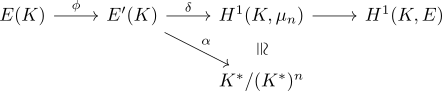
Elliptic Curves - Cambridge III notes

Elliptic Curves
Daniel Naylor

1Fermat’s Method of Infinite Descent
1.1A variant for polynomials
2Some Remarks on Plane Curves
2.1The degree of a morphism
3Weierstrass Equations
4The Group Law
5Isogenies
6The Invariant Differential
7Elliptic Curves over Finite Fields
7.1Zeta functions
8Formal Groups
9Elliptic Curves over Local Fields
10Elliptic Curves over Number Fields: The torsion subgroup
11Kummer Theory
12Elliptic Curves over Number Fields: The weak Mordell-Weil Theorem
13Heights
14Dual isogenies and the Weil pairing
15Galois Cohomology
16Descent by Cyclic Isogeny
16.1Descent by 2-isogeny
16.2Birch Swinnerton Dyer Conjecture
Index

1 Fermat’s Method of Infinite Descent

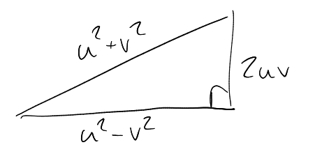
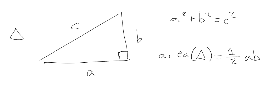
Definition (Rational, primitive triangle). A triangle is rational if $a, b, c \in ℚ$ .

A triangle is primitive if $a, b, c \in ℤ$ and are coprime.

Lemma 1.1. Assuming that:

$Δ$ is a primitive triangle

Then

Δ

is of the form

for some integers $u > v > 0$ .

Proof. Without loss of generality $a$ odd, $b$ even (work modulo $4$ ). This then forces $c$ odd.

Then

{(\frac{b}{2})}^{2} = \frac{c + a}{2} \cdot \frac{c - a}{2},

and note that all the fractions are integers. Also note that the product on the right hand side is a product of positive coprime integers.

Unique prime factorisation in $ℤ$ gives that $\frac{c + a}{2} = u^{2}$ , $\frac{c - a}{2} = v^{2}$ for some $u, v \in ℤ$ .

Then $a = u^{2} - v^{2}$ , $b = 2 u v$ , $c = u^{2} + v^{2}$ . □

Definition (Congruent number). $D \in ℚ_{> 0}$ is a congruent number if there exists a rational triangle $Δ$ with $area (Δ) = D$ .

Note. It suffices to consider $D \in ℤ_{> 0}$ square-free.

Example. $D = 5, 6$ are congruent.

Lemma 1.2. Assuming that:

$D \in ℚ_{> 0}$

Then

D

is congruent if and only if

D y^{2} = x^{3} - x

for some

x, y \in ℚ

y \neq 0

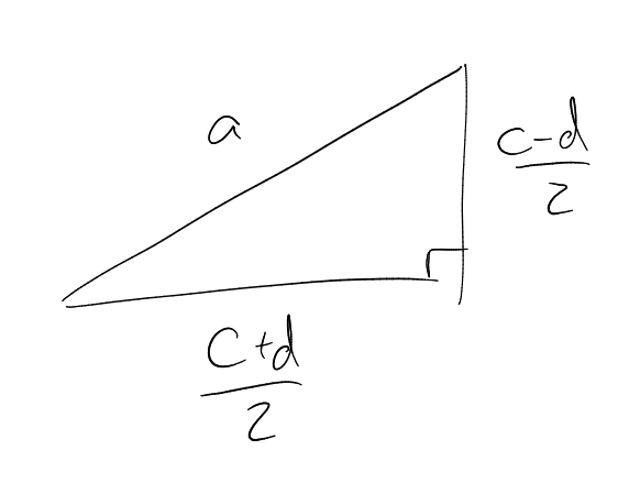
Proof. Lemma 1.1 shows

D congruent ⟺ D w^{2} = u v (u^{2} - v^{2})

for some $u, v, w \in ℚ$ , with $w \neq 0$ . Put $x = \frac{u}{v}$ and $y = \frac{w}{v^{2}}$ . □

Fermat showed that $1$ is not a congruent number.

Theorem 1.3. There is no solution to

w^{2} = u v (u + v) (u - v) (∗)

for $u, v, w \in ℤ$ and $w \neq 0$ .

Proof. Without loss of generality $u, v$ are coprime, $u > 0$ , $w > 0$ . If $v < 0$ then replace $(u, v, w)$ by $(- v, u, w)$ . If $u, v$ both odd then replace $(u, v, w)$ by $(\frac{u + v}{2}, \frac{u - v}{2}, \frac{w}{2})$ .

Then $u, v, u + v, u - v$ are pairwise coprime positive integers with product a square.

Unique factorisation in $ℤ$ gives

u = a^{2}, v = b^{2}, u + v = c^{2}, u - v = d^{2}

for some $a, b, c, d \in ℤ_{> 0}$ .

Since $u ⁄ \equiv v (m o d 2)$ , both $c$ and $d$ are odd.

Then consider:

{(\frac{c + d}{2})}^{2} + {(\frac{c - d}{2})}^{2} = \frac{c^{2} + d^{2}}{2} = u = a^{2} .

This is a primitive triangle. The area is $\frac{c^{2} - d^{2}}{8} = \frac{v}{4} = {(\frac{b}{2})}^{2}$ .

Let $w_{1} = \frac{b}{2}$ . Lemma 1.1 gives $w_{1}^{2} = u_{1} v_{1} (u_{1} + v_{1}) (u_{1} - v_{1})$ for $u_{1}, v_{1} \in ℤ$ . Therefore we have a new solution to ( $*$ ). But $4 w_{1}^{2} = b^{2} = v | w^{2}$ so $w_{1} \leq \frac{1}{2} w$ .

So by Fermat’s method of infinite descent, there is no solution to ( $*$ ) . □

1.1 A variant for polynomials

In Section 1, $K$ is a field with $char K \neq 2$ .

Write $\bar{K}$ for the algebraic closure of $K$ .

Lemma 1.4. Assuming that:

$u, v \in K [t]$ coprime
$α u + β v$ is a square for $4$ distinct $(α : β) \in ℙ^{1}$

Then

u, v \in K

Proof. Without loss of generality $K = \bar{K}$ .

Changing coordinates on $ℙ^{1}$ , we may assume the ratios $(α : β)$ are $(1 : 0), (0 : 1), (1 : - 1), (1 : - λ)$ for some $λ \in K ∖ {0, 1}$ (Möbius map).

\begin{array}{l} u & = a^{2} \\ v & = b^{2} \\ u - v & = (a + b) (a - b) \\ u - λ v & = (a + μ b) (a - μ b) \end{array}

(where $μ$ is a square root of $λ$ ). Unique factorisation in $K [t]$ gives that $a + b$ , $a - b$ , $a + μ b$ , $a - μ b$ are squares. But

\max (\deg (a), \deg (b)) \leq \frac{1}{2} \max (\deg (u), \deg (v)) .

So Fermat’s method of infinite descent, we get a contradiction, unless the degrees of $u$ and $v$ are zero. So $u, v \in K$ . □

Definition 1.5 (Elliptic curve (temporary definition)).

(i) An elliptive curve

E ∕ K

is the projective closure of the plane affine curve

y^{2} = f (x)

where $f \in K [x]$ is a monic cubic polynomial with distinct roots in $\bar{K}$ . We call this equation “a Weierstrass equation”.

(ii) For $L ∕ K$ any field extension
$E (L) = {(x, y) \in L^{2} | y^{2} = f (x)} \cup {0} .$

$0$ is the “point at infinity” that we get because we take the projective closure.

Fact: $E (L)$ is naturally an abelian group.

In this course, we study $E (K)$ for $K$ being a finite field, local field ( $[K : ℚ_{p}] < \infty$ ) or number field ( $[K : ℚ] < \infty$ ).

Lemma 1.2 and Theorem 1.3 tells us that if $E$ is $y^{2} = x^{3} - x$ , then

E (ℚ) = {0, (0, 0), (\pm 1, 0)} .

Corollary 1.6. Let $E ∕ K$ be an elliptic curve. Then $E (K (t)) = E (K)$ .

Proof. Without loss of generality $K = \bar{K}$ . By a change of coordinates, we may assume

y^{2} = x (x - 1) (x - λ)

for some $λ \in K ∖ {0, 1}$ . Suppose $(x, y) \in E (K (t))$ . Put $x = \frac{u}{v}$ , where $u, v \in K [t]$ are coprime.

Then $w^{2} = u v (u - v) (u - λ v)$ for some $w \in K [t]$ .

Unique factorisation in $K [t]$ gives that $u, v, u - v, u - λ v$ are squares. Hence by Section 1.1, $u, v \in K$ , so $x \in K$ , so $y \in K$ . □

2 Some Remarks on Plane Curves

Work over $K = \bar{K}$ .

Definition 2.1 (Rational plane affine curve). A plane affine curve $C = {f (x, y) = 0} \subset 𝔸^{2}$ is rational if it has a rational parametrisation, i.e. $\exists ϕ (t), ψ (t) \in K (t)$ such that:

(i) $𝔸^{1} \to 𝔸^{2}$ , $t \mapsto (ϕ (t), ψ (t))$ is injective on $𝔸^{1} ∖ {finite set}$ .
(ii) $f (ϕ (t), ψ (t)) = 0$ .

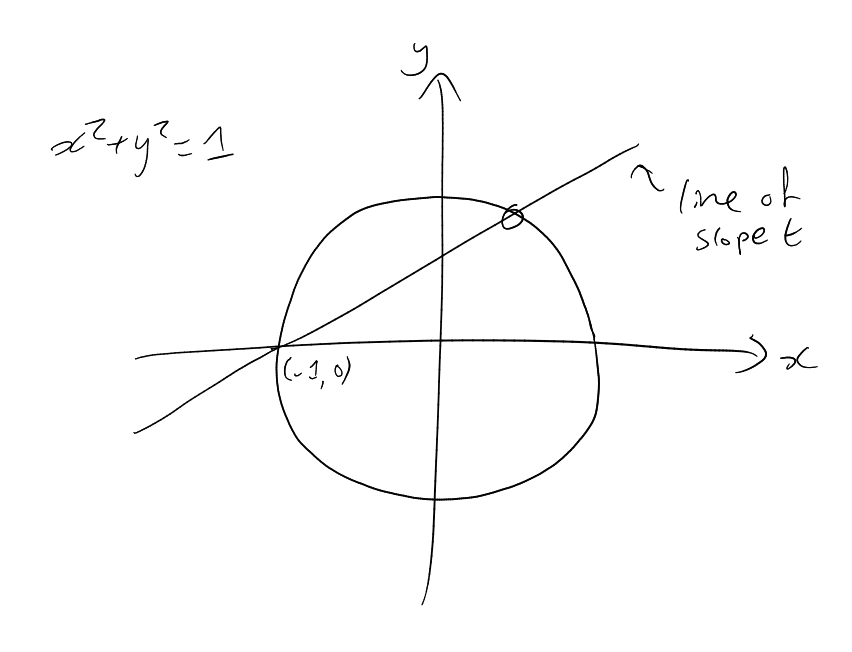
Example 2.2.

(a) Any (non-singular) plane conic is rational.

Substitute $y = t (x + 1)$ . We get $x^{2} + t^{2} {(x + 1)}^{2} = 1$ , hence $(x + 1) ((x - 1) + t^{2} (x + 1)) = 0$ , hence $x = - 1$ or $x = \frac{1 - t^{2}}{1 + t^{2}}$ .

Therefore this has a rational parametrisation
$(x, y) = (\frac{1 - t^{2}}{1 + t^{2}}, \frac{2 t}{1 + t^{2}}) .$
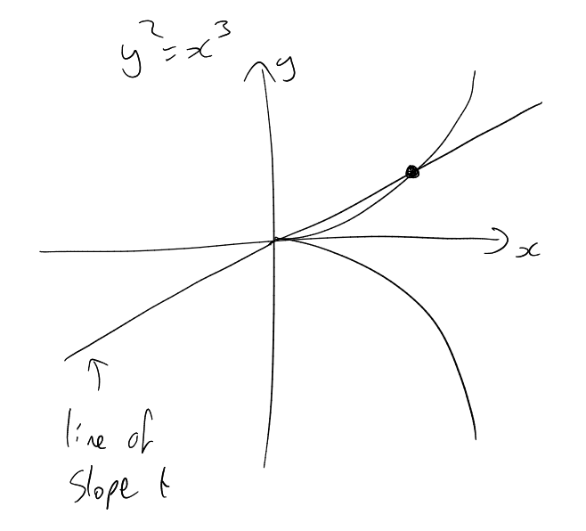
(b) Any singular plane cubic is rational

rational parametrisation $(x, y) = (t^{2}, t^{3})$ .

rational parametrisation: $(x, y) = (e x e r c i s e, e x e r c i s e)$ .
(c) Corollary 1.6 shows that elliptic curves are not rational.

Remark 2.3. The genus $g (C) \in ℤ_{\geq 0}$ is an invariant of a smooth projective curve $C$ .

If $K = ℂ$ then $g (C) = genus of Riemann surface$ .
A smooth plane curve $C \subset ℙ^{2}$ of degree $d$ has genus $g (C) = \frac{(d - 1) (d - 2)}{2}$ .

Proposition 2.4. Assuming that:

$K = \bar{K}$
$C$ a smooth projective curve

Then

(i) $C$ is rational (see Definition 2.1) if and only if $g (C) = 0$ .
(ii) $C$ is an elliptic curve (see Definition 1.5) if and only if $g (C) = 1$ .

Proof.

(i) Omitted.
(ii) $\Rightarrow$ : Check $C$ a smooth plane curve (exercise). Then use Remark 2.3.
$\Leftarrow$ : See later.

□

Order of vanishing

$C$ algebraic curve, function field $K (C)$ , $P \in C$ smooth point.

We write ${ord}_{p} (f)$ for the order of vanishing of $f \in K {(C)}^{\times}$ at $P$ (negative of $f$ has a pole).

Fact: ${ord}_{p} : K {(C)}^{\times} \to ℤ$ is a discrete valuation, i.e. ${ord}_{p} (f_{1} f_{2}) = {ord}_{p} (f_{1}) + {ord}_{p} (f_{2})$ and ${ord}_{p} (f_{1} + f_{2}) \geq \min ({ord}_{p} (f_{1}), {ord}_{p} (f_{2}))$ .

Definition (Uniformiser). $t \in K {(C)}^{\times}$ is a uniformiser at $P$ if ${ord}_{p} (t) = 1$ .

Example 2.5. $C = {g = 0} \subset 𝔸^{2}$ , $g \in K [x, y]$ irreducible.

$K (C) = Frac \frac{K [x, y]}{(g)}$ .

g = g_{0} + g_{1} (x, y) + g_{2} (x, y) + \dots

where $g_{i}$ are homogeneous of degree $i$ .

Suppose $P = (0, 0) \in C$ is a smooth point, i.e. $g_{0} = 0$ , $g_{1} (x, y) = α x + β y$ with $α, β$ not both zero.

Fact: $γ x + δ y \in K (C)$ is a uniformiser at $P$ if and only if $α δ - β γ \neq 0$ .

Example 2.6.

{y^{2} = x (x - 1) (x - λ)} \subset 𝔸^{2}

where $λ \neq 0, 1$ . Projective closure ( $x = \frac{X}{Z}$ , $y = \frac{Y}{Z}$ ):

{Y^{2} Z = X (X - Z) (X - λ Z)} \subset ℙ^{2} .

Let $P = (0 : 1 : 0)$ .

Aim: Compute ${ord}_{p} (x)$ and ${ord}_{p} (y)$ .

Put $w = \frac{Z}{Y}$ , $t = \frac{X}{Y}$ . So

w = t (t - w) (t - λ w) (∗)

Now $P$ is the point $(t, w) = (0, 0)$ . This is a smooth point with

{ord}_{p} (t) = {ord}_{p} (t - w) = {ord}_{p} (t - λ w) = 1 .

( $*$ ) implies ${ord}_{p} (w) = 3$ . Therefore ${ord}_{p} (x) = {ord}_{p} (t ∕ w) = 1 - 3 = - 2$ and ${ord}_{p} (y) = {ord}_{p} (1 ∕ w) = - 3$ .

Riemann Roch Spaces

Let $C$ be a smooth projective curve.

Definition (Divisor). A divisor is a formal sum of points on $C$ , say

D = \sum_{P \in C} n_{p} P

where $n_{p} \in ℤ$ and $n_{p} = 0$ for all but finitely many $P \in C$ .

We write $\deg D = \sum n_{P}$ .

We say $D$ is effective (written $D \geq 0$ ) if $n_{P} \geq 0$ for all $P$ .

If $f \in K {(C)}^{\times}$ , then $div (f) = \sum_{P \in C} {ord}_{p} (f) P$ .

The Riemann Roch space of $D \in Div (C)$ is

L (D) = {f \in K {(C)}^{\times} | div (f) + D \geq 0} \cup {0},

i.e. the $K$ -vector space of rational functions on $C$ with “poles no worse than specified by $D$ ”.

We quote: Riemann Roch for genus $1$ :

\dim L (D) = {\begin{matrix} \deg D & if \deg D > 0 \\ 0 or 1 & if \deg D = 0 \\ 0 & if \deg D < 0 \end{matrix}

For example, in Example 2.6:

\begin{array}{l} L (2 P) & = ⟨ 1, x ⟩ \\ L (3 P) & = ⟨ 1, x, y ⟩ \end{array}

Proposition 2.7. Assuming that:

$K = \bar{K}$ , $char K \neq 2$
$C \subset ℙ^{2}$ a smooth plane cubic
$P \in C$ a point of inflection

Then we may change coordinates such that

C : Y^{2} Z = X (X - Z) (X - λ Z)

for some $λ \neq 0, 1$ and $P = (0 : 1 : 0)$ .

Proof. We change coordinates such that $P = (0 : 1 : 0)$ , $T_{p} (C) = {Z = 0}$ , and $C : {F (X, Y, Z) = 0} \subset ℙ^{2}$ .

$P \in C$ part of inflection implies $F (t, 1, 0) = const t^{3}$ , i.e. $F$ has no terms $X^{2} Y$ , $X Y^{2}$ or $Y^{3}$ .

Therefore

F \in ⟨ Y^{2} Z, X Y Z, Y Z^{2}, X^{3}, X^{2} Z, X Z^{2}, Z^{3} ⟩ .

The $Y^{2} Z$ coefficient must be $\neq 0$ otherwise $P \in C$ is singular, and the coefficient of $X^{3}$ is $\neq 0$ otherwize $Z | F$ .

We are free to rescale $X$ , $Y$ , $Z$ and $F$ . Then without loss of generality $C$ is defined by

Y^{2} Z + a_{1} X Y Z + a_{3} Y Z^{2} = X^{3} + a_{2} X^{z} Z + a_{4} X Z^{2} + a_{6} Z^{3} .

Weierstrass form.

Substituting $Y \leftarrow Y - \frac{1}{2} a_{1} X - \frac{1}{2} a_{3} Z$ , we may suppose $a_{1} = a_{3} = 0$ . Now

Y^{2} Z = Z^{3} f (\frac{X}{Z})

for some monic cubic polynomial $f$ .

$C$ is smooth, so $f$ has distinct roots. Without loss of generality say $0, 1, λ$ . Then $C$ is given by

Y^{2} Z = X (X - Z) (X - λ Z) . □

Remark. It may be shown that the points of inflection on a smooth plane curve

C = {F (X_{1}, X_{2}, X_{3}) = 0} \subset ℙ^{2}

are given by

F = \underset{Hessian}{\underset{⏟}{\det (\frac{\partial^{2} F}{\partial X_{i} \partial X_{j}})}} = 0,

2.1 The degree of a morphism

Let $ϕ : C_{1} \to C_{2}$ be a non-constant morphism of smooth projective curves.

Then $ϕ^{*} : K (C_{2}) \to K (C_{1})$ , $f \mapsto f \circ ϕ$ .

Definition (Degree of a morphism). $\deg ϕ [K (C_{1}) : ϕ^{*} K (C_{2})]$ .

Definition (Separable morphism). $ϕ$ is separable if $K (C_{1}) ∕ ϕ^{*} K (C_{2})$ is a separable field extension.

Definition (Ramification index). Suppose $P \in C_{1}$ , $Q \in C_{2}$ , $ϕ : P \mapsto Q$ . Let $t \in K (C_{2})$ be a uniformiser at $Q$ .

The ramification index of $ϕ$ at $P$ is

e_{ϕ} (P) = {ord}_{P} (ϕ^{*} t)

(always $\geq 1$ , independent of choice of $t$ ).

Theorem 2.8. Assuming that:

$ϕ : C_{1} \to C_{2}$ a non-constant morphism of smooth projective curves

Then

\sum_{P \in ϕ^{- 1} Q} e_{ϕ} (P) = \deg ϕ \forall Q \in C_{2} .

Moreover, if $ϕ$ is separable then $e_{ϕ} (P) = 1$ for all but finitely many $P \in C_{1}$ . In particular:

(i) $ϕ$ is surjective (on $\bar{K}$ -points)
(ii) $# ϕ^{- 1} (Q) \leq \deg ϕ$
(iii) If $ϕ$ is separable then equality holds in (ii) for all but finitely many $Q \in C_{2}$ .

Remark 2.9. Let $C$ be an algebraic curve. A rational map is given $C --\to ℙ^{n}$ , $P \mapsto (f_{0} (P) : f_{1} (P) : \dots : f_{n} (P))$ where $f_{0}, f_{1}, \dots, f_{n} \in K (C)$ are not all zero.

Important Fact: If $C$ is smooth then $ϕ$ is a morphism.

3 Weierstrass Equations

In this section, we drop the assumption that $K = \bar{K}$ , but we instead assume that $K$ is a perfect field.

Definition (Elliptic curve). An elliptic curve $E ∕ K$ is a smooth projective curve of genus $1$ , defined over $K$ with a specified $K$ -rational point $0_{E} \in E (K)$ .

Example. ${X^{3} + p Y^{3} + p^{2} Z^{3} = 0} \subset ℙ^{2}$ is not an elliptic curve over $ℚ$ , since it has no $ℚ$ -rational points.

Theorem 3.1. Assuming that:

$E$ is an elliptic curve

Then

E

is isomorphic over

K

to a curve in Weierstrass form via an isomorphism taking

0_{E}

(0 : 1 : 0)

Remark. Proposition 2.7 treated the special case $E$ is a smooth plane cubic and $0_{E}$ is a point of inflection.

Fact: If $D \in Div (E)$ is defined over $K$ (i.e. fixed by $Gal (\bar{K} ∕ K)$ ) then $L (D)$ has a basis in $K (E)$ (not just $\bar{K} (E)$ ).

Proof of Theorem 3.1. $L (2 . 0_{E}) \subset L (3 . 0_{E})$ . Pick basis $1, x$ for $L (2 . 0_{E})$ and $1, x, y$ for $L (3 . 0_{E})$ .

Note: ${ord}_{0_{E}} (x) = - 2$ , ${ord}_{0_{E}} (y) = - 3$ .

The 7 elements $1, x, y, x^{2}, x y, x^{3}, y^{2}$ in the 6-dimensional space $L (6 . 0_{E})$ must satisfy a dependence relation.

Leaving out $x^{3}$ or $y^{2}$ gives a basis for $L (6 . 0_{E})$ since each term has a different order pole at $0_{E}$ .

Therefore the coefficients of $x^{3}$ and $y^{2}$ are non-zero. Rescaling $x$ and $y$ (if necessary) we get

y^{2} + a_{1} x y + a_{3} y = x^{3} + a_{2} x^{2} + a_{4} x + a_{6}

for some $a_{i} \in K$ .

Let $E^{'}$ be the curve defined by this equation (or rather its projective closure). There is a morphism

\begin{array}{l} ϕ : E & \to E^{'} \subset ℙ^{2} \\ P & \mapsto (x (P) : y (P) : 1) = (\frac{x}{y} (P) : 1 : \frac{1}{y} (P)) \\ 0_{E} & \mapsto (0 : 1 : 0) \end{array}

Then

\begin{array}{l} [K (E) : K (x)] & = \deg (E \overset{x}{\to} ℙ^{1}) \\ = {ord}_{0_{E}} (\frac{1}{x}) \\ = 2 [K (E) : K (y)] & = \deg (E \overset{y}{\to} ℙ^{1}) \\ = {ord}_{0_{E}} (\frac{1}{y}) \\ = 3 \end{array}

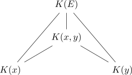
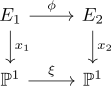
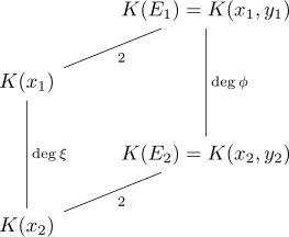
This gives us a diagram of field extensions:

By the Tower Law (since

2, 3

are coprime), we get that

[K (E) : K (x, y)] = 1

. Hence

K (E) = K (x, y) = ϕ^{*} K (E^{'})

, so

\deg ϕ = 1

, so

ϕ

is birational.

If $E^{'}$ is singular then $E$ and $E^{'}$ are rational, contradiction.

So $E^{'}$ is smooth. Then Remark 2.9 implies that $ϕ^{- 1}$ is a morphism. So $ϕ$ is an isomorphism. □

Proposition 3.2. Assuming that:

$K$ is perfect
$E$ , $E^{'}$ are elliptic curves over $K$
$E, E^{'}$ are in Weierstrass form

Then

E ≅ E^{'}

over

K

if and only if the equations are related by a change of variables

\begin{array}{l} x & = u^{2} x^{'} + r \\ y & = u^{3} y^{'} + u^{2} s x^{'} + t \end{array}

where $u, r, s, t \in K$ with $u \neq 0$ .

Proof.

$\Leftarrow$ Obvious.
$\Rightarrow$ $⟨ 1, x ⟩ = L (2 . 0_{E}) = ⟨ 1, x^{'} ⟩$ hence $x = λ x^{'} + r$ for some $λ, r \in K$ with $λ \neq 0$ .
$⟨ 1, x, y ⟩ = L (3 . 0_{E}) = ⟨ 1, x^{'}, y^{'} ⟩$ implies $y = μ y^{'} + σ x^{'} + t$ for some $μ, σ, t \in K$ with $μ \neq 0$ .

Looking at coefficients of $x^{3}$ and $y^{2}$ , we get $λ^{3} = μ^{2}$ . So $λ = u^{2}$ , $μ = u^{3}$ for some $0 \neq u \in K$ .

Put $s = \frac{σ}{u^{2}}$ . □

A Weierstrass form equation defines an elliptic curve if and only if it defines a smooth curve, which happens if and only if $Δ (a_{1}, \dots, a_{6}) \neq 0$ , where $Δ \in ℤ [a_{1}, \dots, a_{6}]$ is a certain polynomial.

If $char K \neq 2, 3$ , we may reduce to the case $E : y^{2} = x^{3} + a x + b$ , with discriminant $Δ = - 16 (4 a^{3} + 27 b^{2})$ .

Corollary 3.3. Assuming that:

$char K \neq 2, 3$ and $K$ is perfect
elliptic curves $E : y^{2} = x^{3} + a x + b$ , $E^{'} : y^{2} = x^{3} + a^{'} x + b^{'}$

Then

E

and

E^{'}

are isomorphic over

K

if and only if

a^{'} = u^{4} a

b^{'} = u^{6} b

for some

u \in K^{*}

Proof. $E$ and $E^{'}$ are related by a substitution as in Proposition 3.2 with $r = s = t = 0$ . □

Definition ( $j$ -invariant). The $j$ -invariant is

j (E) = \frac{1728 (4 a^{3})}{4 a^{3} + 27 b^{2}} .

Corollary 3.4. Assuming that:

$E ≅ E^{'}$

Then

j (E) = j (E^{'})

. Moreover, the converse holds if

K = \bar{K}

Proof.

\begin{array}{l} E ≅ E^{'} & ⟺ {\begin{matrix} a^{'} = u^{4} a \\ b^{'} = u^{6} b \end{matrix} for some u \in K^{*} \\ ⟹ (a^{3} : b^{2}) = ({(a^{'})}^{3} : {(b^{'})}^{2}) \\ ⟺ j (E) = j (E^{'}) \end{array}

and the converse holds if $K = \bar{K}$ (to go backwards on the $⟹$ step, we only need to take some kind of $n$ -th root). □

4 The Group Law

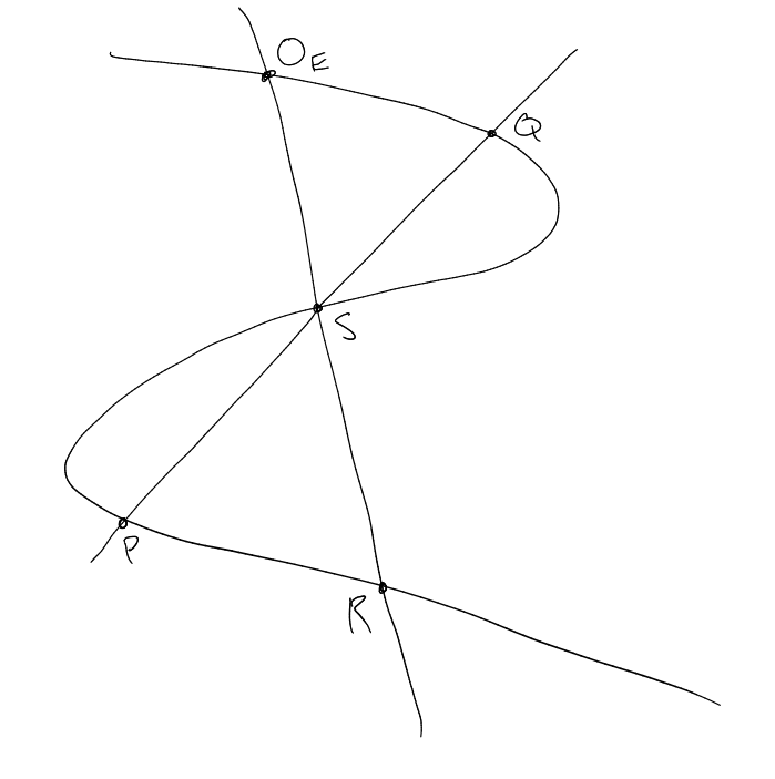
Let $E \subset ℙ^{2}$ be a smooth plane cubic, and $0_{E} \in E (K)$ .

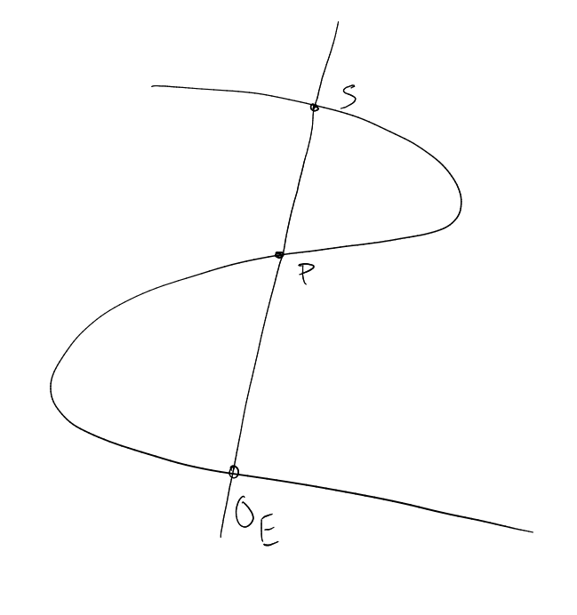
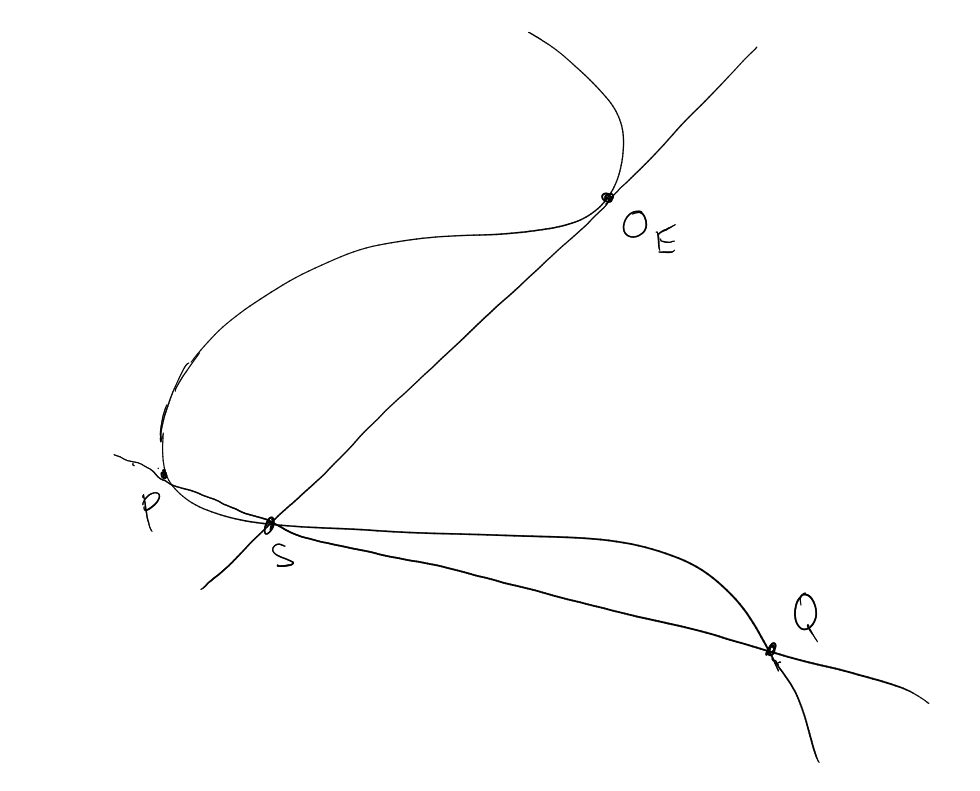
$E$ meets any line in 3 points counted with multiplicity.

Let $S$ be the third point of intersection of $P Q$ with $E$ , and $R$ be the third intersection point of $0_{E} S$ and $E$ .

Define $P \oplus Q = R$ .

If $P Q$ then take $T_{P} E$ instead of $P Q$ etc.

This is called the “chord and tangent process”.

Theorem 4.1. $(E, \oplus)$ is an abelian group.

Note. $E$ here means $E (\bar{K})$ . As mentioned before, we only ever mean “over $K$ ” if it is explicitly mentioned (otherwise we are always working “over $\bar{K}$ ”).

Proof.

(i) $\oplus$ is clearly commutative.
(ii) $0_{E}$ is the identity:

$0_{E} \oplus P = P$ .
(iii) Inverses:

Let $S$ be the third point of intersection of $T_{0_{E}} E$ and $E$ , and let $Q$ be the third point of intersection of $P S$ and $E$ .

Then $P \oplus Q = 0_{E}$ .
(iv) Associativity: much harder! We will develop a bit of theory first. □

Definition (Linearly equivalent). $D_{1}, D_{2} \in Div (E)$ are linearly equivalent if there exists $f \in \bar{K} {(E)}^{*}$ such that $div (f) = D_{1} - D_{2}$ .

Write $D_{1} \sim D_{2}$ and $[D] = {D^{'} : D^{'} \sim D}$ .

Definition. $Pic (E) = \frac{Div (E)}{\sim}$ , ${Pic}^{0} (E) = \frac{{Div}^{0} (E)}{\sim}$ . where ${Div}^{0} (E) = {D \in Div E | \deg D = 0}$ .

Proposition 4.2. Assuming that:

we define
$\begin{array}{l} ψ : E & \to {Pic}^{0} (E) \\ P & \mapsto [(P) - (0_{E})] \end{array}$

Then

(i) $ψ (P \oplus Q) = ψ (P) + ψ (Q)$ .
(ii) $ψ$ is a bijection.

Proof.

(i) $\begin{array}{l} div (l ∕ m) & = (P) + (S) + (Q) - (0_{E}) - S - (R) \\ = (P) + (Q) - (0_{E}) - (P \oplus Q) \end{array}$
Hence $(P) + (Q) \sim (P \oplus Q) + (0_{E})$ . Therefore $(P \oplus Q) - (0_{E}) \sim (P) - (0_{E}) + (Q) - (0_{E})$ . So $ψ (P \oplus Q) = ψ (P) + ψ (Q)$ .
(ii) Injectivity: Suppose $ψ (P) = ψ (Q)$ with $P \neq Q$ .
Then there exists $f \in \bar{K} {(E)}^{*}$ such that $div (f) = (P) - (Q)$ , so $E \overset{f}{\to} ℙ^{1}$ has degree 1, hence $E ≅ ℙ^{1}$ , contradiction.

Note: We now compute
$ψ ((P \oplus Q) \oplus R) = ψ (P) + ψ (Q) + ψ (R) = ψ (P \oplus (Q \oplus R))$

hence $(P \oplus Q) \oplus R = P \oplus (Q \oplus R)$ for all $P, Q, R \in E$ (using injectivity). So $(E, \oplus)$ is associative.

(iii) Surjectivity: Let

[D] \in {Pic}^{0} (E)

. Then

D + (0_{E})

has degree

1

Riemann Roch gives $\dim L (D + (0_{E})) = 1$ . So there exists $0 \neq f \in \bar{K} (E)$ such that

\underset{degree 1}{\underset{⏟}{div (f) + D + (0_{E})}} \geq 0 .

div (f) + D + (0_{E}) = (P)

for some $P \in E$ . Then $(P) - (0_{E}) \sim D$ , so $ψ (P) = [D]$ . □

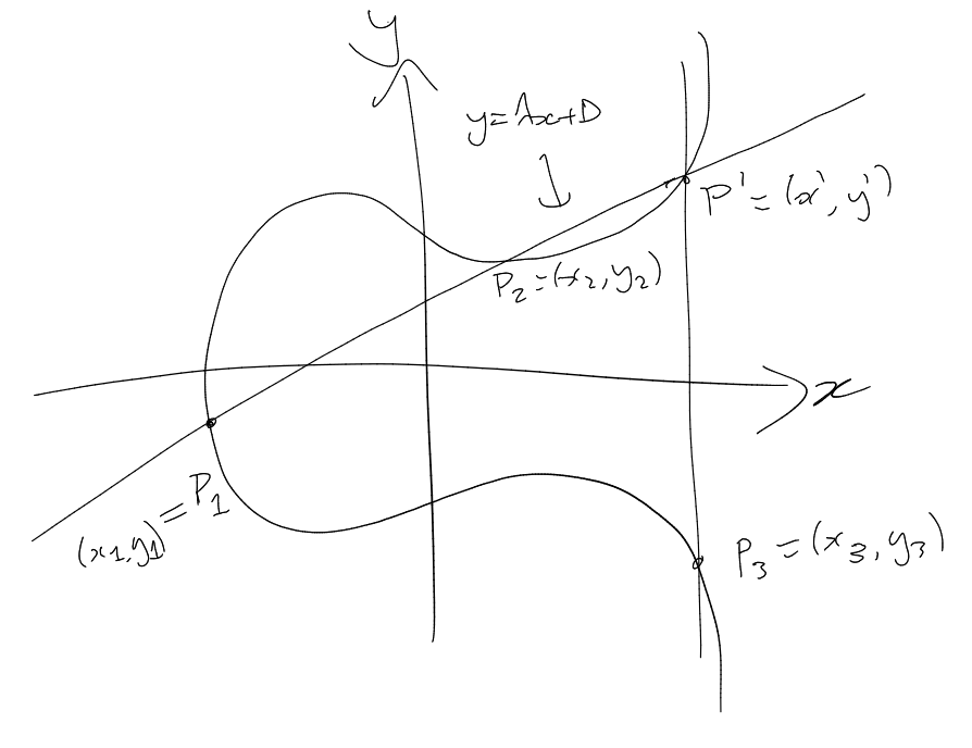
Formulae for $E$ in Weierstrass form

E : y^{2} + a_{1} x y + a_{3} y = x^{3} + a_{2} x^{2} + a_{4} x + a_{6} (∗)

$0_{E} = (0 : 1 : 0)$ .

$P_{1} \oplus P_{2} = P_{3}$ . $⊖ P_{1} = (x_{1}, - (a_{1} x + a_{3}) - y_{1})$ .

Substituting $y = λ x + ν$ into ( $*$ ) and looking at coefficient of $x^{2}$ gives

λ^{2} + a_{1} λ - a_{2} = x_{1} + x_{2} + \underset{= x_{3}}{\underset{⏟}{x^{'}}} .

Therefore

\begin{array}{l} x_{3} & = λ^{2} + a_{1} λ - a_{2} - x_{1} - x_{2} \\ y_{3} & = - (a_{1} x^{'} + a_{3}) - y^{'} \\ = - (a_{1} x_{3} + a_{3}) - (λ x_{3} + ν) \\ = - (λ + a_{1}) x_{3} - a_{3} - ν \end{array}

It remains to find formulae for $λ$ and $ν$ .

Case I $x_{1} = x_{2}$ , $P_{1} \neq P_{2}$ . Then $P_{1} \oplus P_{2} = 0_{E}$ .
Case II $x_{1} \neq x_{2}$ . $\begin{array}{l} λ & = \frac{y_{2} - y_{1}}{x_{2} - x_{1}} \\ ν & = y_{1} + λ x_{1} \\ = \frac{y_{1} (x_{2} - x_{1}) - x_{1} (y_{2} - y_{1})}{x_{2} - x_{1}} \\ = \frac{x_{2} y_{1} - x_{1} y_{2}}{x_{2} - x_{1}} \end{array}$
Case III $P_{1} = P_{2}$ . $\begin{array}{l} λ & = \dots \\ ν & = \dots \end{array}$
(Compute equation for tangent line.)

Corollary 4.3. $E (K)$ is an abelian group.

Proof. It is a subgroup of $(E, \oplus)$ . Identity $0_{E} \in E (K)$ by definition.

Closure / inverses: see formulae above.

Associative / commutative: inherited. □

Theorem 4.4. Elliptic curves are group varieties, i.e. $[- 1] : E \to E$ ; $P \mapsto ⊖ P$ and $\oplus : E \times E \to E$ ; $(P, Q) \mapsto P \oplus Q$ are morphisms of algebraic varieties.

Proof.

(i) Above formulae imply $[- 1] : E \to E$ is a rational map, and hence a morphism (by Remark 2.9).

(ii) Above formulae imply

\oplus : E \times E \to E

is a rational map regular on

U = {(P, Q) \in E \times E | P, Q, P \oplus Q, P ⊖ Q \neq 0_{E}} .

For $P \in E$ , let $τ_{P} : E \to E$ ; $X \mapsto X \oplus P$ “translation by $P$ ”.

$τ_{P}$ is a rational map, and hence a morphism (by Remark 2.9).

Take any $A, B \in E$ . We factor $\oplus$ as

E \times E \overset{τ_{⊖ A} \times τ_{⊖ B}}{\to} E \times E \overset{\oplus}{\to} E \overset{τ_{A \oplus B}}{\to} E .

This shows $\oplus$ is regular on $(τ_{A} \times τ_{B}) (U)$ for all $A, B \in E$ . Therefore $\oplus$ is regular on $E \times E$ . □

Statement of Results

The isomorphisms in (i), (ii), (iv) respect the relevant topologies.

(i) $K = ℂ$ , $E (ℂ) = ℂ ∕ Λ ≅ ℝ ∕ ℤ \times ℝ ∕ ℤ$ ( $Λ$ is a lattice).
(ii) $K = ℝ$ . Then
$E (ℝ) = {\begin{matrix} ℤ ∕ 2 ℤ \times ℝ ∕ ℤ & if Δ > 0 \\ ℝ ∕ ℤ & if Δ < 0 \end{matrix}$
(iii) $K = 𝔽_{q}$ (field with $q$ elements). Then
$| # E (𝔽_{q}) - (q + 1) | \leq 2 \sqrt{q} .$

(Hasse’s Theorem).
(iv) $[K : ℚ_{p}] < \infty$ , ring of integers $O_{K}$ . $E (K)$ has a subgroup of finite index which is isomorphic to $(O_{K}, +)$ .
(v) $[K : ℚ] < \infty$ . $E (K)$ is a finitely generated abelian group (Mordell-Weil Theorem).

Brief remarks on the case $K = ℂ$

Let

Λ = {a ω_{1} + b ω_{2} : a, b \in ℤ},

where $ω_{1}, ω_{2}$ a basis for $ℂ$ as an $ℝ$ -vector space.

Then

{meromorphic functions on the Riemann surface ℂ ∕ Λ} \leftrightarrow {Λ -invariant meromorphic functions on ℂ} .

The function field of $ℂ ∕ Λ$ is generated by

\begin{array}{l} ℘ (z) & = \frac{1}{z^{2}} + \sum_{0 \neq λ \in Λ} (\frac{1}{{(z - λ)}^{2}} - \frac{1}{λ^{2}}) \\ ℘^{'} (z) & = - 2 \sum_{λ \in Λ} \frac{1}{{(z - λ)}^{3}} \end{array}

These satisfy

℘^{'} {(z)}^{2} = 4 ℘ {(z)}^{3} - g_{2} ℘ (z) - g_{3}

for some $g_{2}, g_{3} \in ℂ$ depending only on $Λ$ .

One shows $ℂ ∕ Λ = E (ℂ)$ (isomorphism as groups and as Riemann surfaces) where $E$ : $y^{2} = 4 x^{3} - g_{2} x - g_{3}$ .

Theorem (Uniformisation Theorem). Every elliptic curve over $ℂ$ arises this way (one proof uses modular forms).

Definition. For $n \in ℤ$ , let $[n] : E \to E$ be defined by

P \mapsto \underset{n copies}{\underset{⏟}{P \oplus P \oplus \dots \oplus P}}

for $n \geq 0$ , and $[- n] = [- 1] \circ [n]$ .

Definition ( $n$ -torsion subgroup). The $n$ -torsion subgroup of $E$ is

E [n] = \ker (E \overset{[n]}{\to} E) .

If $K = ℂ$ then $E (ℂ) ≅ ℂ ∕ Λ$ . Therefore

{\begin{matrix} E [n] ≅ {(ℤ ∕ n ℤ)}^{2} & (1) \\ \deg [n] = n^{2} & (2) \end{matrix}

We’ll show (2) holds over any field $K$ , and (1) holds if $char K ∤ n$ .

Lemma 4.5. Assuming that:

$char K \neq 2$
$E$ : $y^{2} = f (x) = (x - e_{1}) (x - e_{2}) (x - e_{3})$ , $e_{1}, e_{2}, e_{3} \in \bar{K}$

Then

E [2] = {0_{E}, (e_{1}, 0), (e_{2}, 0), (e_{3}, 0)} ≅ {(ℤ ∕ 2 ℤ)}^{2}

Proof. Let $P = (x, y) \in E$ . Then

\begin{array}{l} [2] P = 0 & ⟹ P = - P \\ ⟹ (x, y) = (x, - y) \\ ⟹ y = 0 □ \end{array}

5 Isogenies

Let $E_{1}, E_{2}$ be elliptic curves.

Definition (Isogeny). An isogeny $ϕ : E_{1} \to E_{2}$ is a nonconstant morphism with $ϕ (0_{E_{1}}) = 0_{E_{2}}$ (by Theorem 2.8, a morphism is nonconstant if and only if surjective on $\bar{K}$ -points).

We say $E_{1}$ and $E_{2}$ are isogenous in this case.

Definition. $Hom (E_{1}, E_{2}) = {isogenies E_{1} \to E_{2}} \cup {0}$ .

This is an abelian group under

(ϕ + ψ) (P) = ϕ (P) + ψ (P) .

If $E_{1} \overset{ϕ}{\to} E_{2} \overset{ψ}{\to} E_{3}$ are isogenies then $ψ \circ ϕ$ is an isogeny.

Tower Law implies $\deg (ψ ϕ) = \deg (ϕ) \deg (ψ)$ .

Proposition 5.1. Assuming that:

$0 \neq n \in ℤ$

Then

[n] : E \to E

is an isogeny.

Proof. $[n]$ is a morphism by Theorem 4.4. We must show $[n] \neq [0]$ .

Assume $char K \neq 2$ .

Case $n = 2$ : Lemma 4.5 implies $E [2] \neq E$ implies $[2] \neq [0]$ .

Case $n$ odd: Lemma 4.5 implies $\exists 0 \neq T \in E [2]$ . Then $n T = T \neq 0$ which gives $[n] \neq [0]$ .

Now use $[m n] = [m] \circ [n]$ .

If $char K = 2$ , then could rpelace Lemma 4.5 with an explicit lemma about $3$ -torsion points. □

Corollary 5.2. $Hom (E_{1}, E_{2})$ is a torsion free $ℤ$ -module.

Theorem 5.3. Assuming that:

$ϕ : E_{1} \to E_{2}$ an isogeny

Then

ϕ (P + Q) = ϕ (P) + ϕ (Q)

for all

P, Q \in E_{1}

Proof (sketch). $ϕ$ incudes

\begin{array}{l} ϕ_{*} : {Div}^{0} (E_{1}) & \to {Div}^{0} (E_{2}) \\ \sum_{P \in E_{1}} n_{P} P & \mapsto \sum_{P \in E_{1}} n_{P} ϕ (P) \end{array}

Recall $ϕ^{*} : K (E_{2}) ↪ K (E_{1})$ .

Fact: If

f \in \bar{K} {(E_{1})}^{*}

then

div (N_{K (E_{1}) ∕ K (E_{2})} f) = ϕ_{*} (div f) .

So $ϕ_{*}$ sends principal divisors to principal divisors.

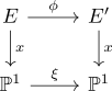
Since $ϕ (0_{E_{1}}) = 0_{E_{2}}$ , the following diagram commutes:

P E1 E2 Q

0 0
ϕ∼=∼=ϕ∗ [(P )− (0E1)] Pic (E1) Pic(E2) [(Q )− (0E2)]

ϕ_{*}

a group homomorphism implies

ϕ

is a group homomorphism. □

Lemma 5.4. Assuming that:

$ϕ : E_{1} \to E_{2}$ an isogeny

Then there exists a morphism

ξ

making the following diagram commute:

(

x_{i} =

x

-coordinate on a Weierstrass equation for

E_{i}

). Moreover if

ξ (t) = \frac{r (t)}{s (t)}

r, s \in K [t]

coprime, then

\deg ϕ = \deg ξ = \max (\deg (r), \deg (s)) .

Proof. For $i = 1, 2$ . $K (E_{i}) ∕ K (x_{i})$ is a degree $2$ Galois extension, with Galois group generated by ${[- 1]}^{*}$ .

Theorem 5.3 implies that $ϕ \circ [- 1] = [- 1] \circ ϕ$ .

So if $f \in K (x_{2})$ then

{[- 1]}^{*} ϕ^{*} f = ϕ^{*} {[- 1]}^{*} f = ϕ^{*} f .

Therefore $ϕ^{*} f \in K (x_{1})$ .

K (E1) = K (x1,y1)

K (x1)

K (E2) = K (x2,y2)

2dd2eeggKϕξ (x2)

In particular,

ϕ^{*} = ξ (x_{1})

for some rational function

ξ

Tower Law implies $\deg ϕ = \deg ξ$ .

Now $K (x_{2}) ↪ K (x_{1})$ , $x_{2} \mapsto ξ (x_{1}) = \frac{r (x_{1})}{s (x_{1})}$ , $r, s \in K [t]$ coprime.

We claim the minimal polynomial of $x_{1}$ over $K (x_{2})$ is

F (t) = r (t) - s (t) x_{2} \in K (x_{2}) [t] .

Check:

$F (x_{1}) = 0$ : true by the definition of our embedding.
$F$ is irreducible in $K [x_{2}, t]$ (since $r, s$ coprime), hence irreducible in $K (x_{2}) [t]$ by Gauss’s lemma.

Therefore

\deg ξ = [K (x_{1}) : K (x_{2})] = \deg F = \max (\deg r, \deg s) . □

Lemma 5.5. $\deg [2] = 4$ .

Proof. Assume $char K \neq 2, 3$ (the result is true even in the case of $char K \in {2, 3}$ , but we will only prove the simpler case).

$E$ : $y^{2} = x^{3} + a x + b = f (x)$ .

If $P = (x, y) \in E$ , then

\begin{array}{l} x (2 P) & = {(\frac{3 x^{2} + a}{2 y})}^{2} - 2 x \\ = \frac{{(3 x^{2} + a)}^{2} - 8 x f (x)}{4 f (x)} \\ = \frac{x^{4} + \dots}{f (x)} \end{array}

The numerator and denominator are coprime. Indeed, otherwise there exists $𝜃 \in \bar{K}$ with $f (𝜃) = f^{'} (𝜃) = 0$ and hence $f$ has a multiple root (contradiction).

Now Lemma 5.4 implies $\deg [2] = \max (4, 3) = 4$ . □

Definition (Quadratic form in an abelian group). Let $A$ be an abelian group. We say $q : A \to ℤ$ is a quadratic form if

(i) $q (n x) = n^{2} q (x)$ for all $n \in ℤ$ , $x \in A$ .
(ii) $(x, y) \mapsto q (x + y) - q (x) - q (y)$ is $ℤ$ -bilinear.

Lemma 5.6. $q : A \to ℤ$ is a quadratic form if and only if it satisfies the parallelogram law:

q (x + y) + q (x - y) = 2 q (x) = 2 q (y) \forall x, y \in A .

Proof.

\Rightarrow

Let

⟨ x, y ⟩ = q (x + y) - q (x) - q (y)

. Then

⟨ x, x ⟩ = q (2 x) - 2 q (x) = 2 q (x)

(the equality in the last step is using property (i) with $n = 2$ ).

But by (ii),

⟨ x + y, x + y ⟩ + ⟨ x - y, x - y ⟩ = 2 ⟨ x, x ⟩ + 2 ⟨ y, y ⟩ .

Hence (upon dividing by $2$ ),

q (x + y) + q (x - y) = 2 q (x) + 2 q (y) .

$\Leftarrow$ See Example Sheet 2. □

Theorem 5.7. $\deg : Hom (E_{1}, E_{2}) \to ℤ$ is a quadratic form.

Note. We define $\deg (0) = 0$ .

For the proof we assume $char K \neq 2, 3$ . Write $E_{2}$ : $y^{2} = x^{3} + a x + b$ .

Let $P, Q \in E_{2}$ with $P, Q, P + Q, P - Q \neq 0$ . Let $x_{1}, \dots, x_{4}$ be the $x$ -coordinates of the $4$ points.

Lemma 5.8. There exists $W_{0}, W_{1}, W_{2} \in ℤ [a, b] [x_{1}, x_{2}]$ of degree in $x_{1}$ and of degree $\leq 2$ in $x_{2}$ such that

(1 : x_{3} + x_{4} : x_{3} x_{4}) = (W_{0} : W_{1} : W_{2}) .

Proof. Two methods.

(1) Direct calculation: $\begin{array}{l} W_{0} & = {(x_{1} - x_{2})}^{2} \\ W_{1} & = \dots \\ W_{2} & = \dots \end{array}$
see formula sheet.

(2) Let

y = λ x + ν

be the line through

P

and

Q

\begin{array}{l} x^{3} + a x + b - {(λ x + ν)}^{2} & = (x - x_{1}) (x - x_{2}) (x - x_{3}) \\ = x^{3} - s_{1} x^{2} + x_{2} x - s_{3} \end{array}

where $s_{i}$ is the $i$ -th elementary symmetric polynomial in $x_{1}, x_{2}, x_{3}$ .

Comparing coefficients:

\begin{array}{l} λ^{2} & = s_{1} \\ - 2 λ ν & = s_{2} - a \\ ν^{2} & = s_{3} + b \end{array}

Eliminating $λ$ and $ν$ gives

\underset{= F (x_{1}, x_{2}, x_{3})}{\underset{⏟}{{(s_{2} - a)}^{2} - 4 s_{1} (s_{3} + b) = 0}}

where $F$ has degree $\leq 2$ in $x_{i}$ .

$x_{3}$ is a root of the quadratic

W (t) = F (x_{1}, x_{2}, t) .

Repeating for the line through $P$ and $- Q$ shows that $x_{4}$ is the other root. Therefore

W_{0} (t - x_{3}) (t - x_{4}) = W_{0} t^{2} - W_{1} t + W_{2},

hence

(1 : x_{3} + x_{4} : x_{3} x_{4}) = (W_{0} : W_{1} : W_{2}) . □

We show that if $ϕ, ψ \in Hom (E_{1}, E_{2})$ , then

\deg (ϕ + ψ) + \deg (ϕ - ψ) \leq 2 \deg (ϕ) + 2 \deg (ψ) .

We may assume $ϕ, ψ, ϕ + ψ, ϕ - ψ \neq 0$ (otherwise trivial, or use $\deg [- 1] = 1$ , $\deg [2] = 4$ ).

\begin{array}{l} ϕ & : (x, y) \mapsto (ξ_{1} (x), \dots) \\ ψ & : (x, y) \mapsto (ξ_{2} (x), \dots) \\ ϕ + ψ & : (x, y) \mapsto (ξ_{3} (x), \dots) \\ ϕ - ψ & : (x, y) \mapsto (ξ_{4} (x), \dots) \end{array}

Lemma 5.8 implies

(1 : ξ_{3} + ξ_{4} : ξ_{3} ξ_{4}) = ({(ξ_{1} - ξ_{2})}^{2} : \dots) .

Put $ξ_{i} = \frac{r_{i}}{s_{i}}$ , $r_{i}, s_{i} \in K [t]$ coprime.

\underset{coprime}{\underset{⏟}{(s_{3} s_{4} : r_{3} s_{4} + r_{4} s_{4} : r_{3} r_{4})}} = ({(r_{1} s_{2} - r_{2} s_{1})}^{2} : \dots) . (∗)

Therefore

\begin{array}{l} \deg (ϕ + ψ) + \deg (ϕ - ψ) & = \max (\deg (r_{3}), \deg (s_{3})) + \max (\deg (r_{4}), \deg (s_{4})) \\ = \max (\deg (s_{3} s_{4}), \deg (r_{3} s_{4} + r_{3} s_{3}), \deg (r_{3} r_{4})) \\ \leq 2 \max (\deg (r_{1}), \deg (s_{1})) + 2 \max (\deg (r_{2}), \deg (s_{2})) \\ = 2 \deg (ϕ) + 2 \deg (ψ) & (1) \end{array}

Now replace $ϕ, ψ$ by $ϕ + ψ, ϕ - ψ$ to get

\begin{array}{l} \deg (2 ϕ) + \deg (2 ψ) & \leq 2 \deg (ϕ + ψ) + 2 \deg (ϕ - ψ) \\ 4 \deg (ϕ) + 4 \deg (ψ) & \leq 2 \deg (ϕ + ψ) + 2 \deg (ϕ - ψ) \\ 2 \deg (ϕ) + 2 \deg (ψ) & \leq \deg (ϕ + ψ) + \deg (ϕ - ψ) & (2) \end{array}

(1) and (2) give that $\deg$ satisfies the parallelogram law, hence $\deg$ is a quadratic form.

This proves Theorem 5.7.

Corollary 5.9. $\deg (n ϕ) = n^{2} \deg (ϕ)$ for all $n \in ℤ$ , $ϕ \in Hom (E_{1}, E_{2})$ . In particular, $\deg [n] = n^{2}$ .

Example 5.10. Let $E ∕ K$ be an elliptic curve. Suppose $char K \neq 2$ . Let $0 \neq T \in E (K) [2]$ .

Without loss of generality $E$ : $y^{2} = x (x^{2} + a x + b)$ , $a, b \in K$ , $b (a^{2} - 4 b) \neq 0$ , and $T = (0, 0)$ .

If $P = (x, y)$ and $P^{'} = P + T = (x^{'}, y^{'})$ then

\begin{array}{l} x^{'} & = {(\frac{y}{x})}^{2} - a - x \\ = \frac{x^{2} + a x + b}{x} - a - x \\ = \frac{b}{x} \\ y^{'} & = (\frac{y}{x}) x^{'} \\ = - \frac{b y}{x} \end{array}

Let

\begin{array}{l} ξ & = x + x^{'} + a = {(\frac{y}{x})}^{2} \\ η & = y + y^{'} = \frac{y}{x} (x - \frac{b}{x}) \\ η^{2} & = {(\frac{y}{x})}^{2} [{(x + \frac{b}{x})}^{2} - 4 b] \\ = ξ [{(ξ - a)}^{2} - 4 b] \\ = ξ (ξ^{2} - 2 a ξ + a^{2} - 4 b) \end{array}

Let $E^{'}$ : $y^{2} = x (x^{2} + a^{'} x + b^{'})$ , where $a^{'} = - 2 a$ , $b^{'} = a^{2} - 4 b$ . There is an isogeny

\begin{array}{l} ϕ : E & \to E^{'} \\ (x, y) & \mapsto ({(\frac{y}{x})}^{2} : \frac{y (x^{2} - b)}{x^{2}} : 1) \\ - 2 - 3 0 {ord}_{0_{E}} (∙) \\ 1 0 3 + 3 \\ 0_{E} & \mapsto (0 : 1 : 0) = 0_{E^{'}} \end{array}

To compute the degree: ${(\frac{y}{x})}^{2} = \frac{x^{2} + a x + b}{x}$ (coprime numerator and denominator as $b \neq 0$ ). Lemma 5.4 gives $\deg ϕ = 2$ .

We say $ϕ$ is a $2$ -isogeny.

6 The Invariant Differential

Let $C$ be an algebraic curve over $K = \bar{K}$ .

Definition (Space of differentials). The space of differentials $Ω_{C}$ is the $K (C)$ -vector space generated by $d f$ for $f \in K (C)$ , subject to the relations

(i) $d (f + g) = d f + d g$
(ii) $d (f g) = f d g + g d f$
(iii) $d a = 0 \forall a \in K$

Fact: $Ω_{C}$ is a $1$ -dimensional $K (C)$ -vector space.

Let $0 \neq ω \in Ω_{C}$ . Let $P \in C$ be a smooth point, and $t \in K (C)$ a uniformiser at $P$ .

Then $ω = f d t$ for some $f \in K {(C)}^{*}$ . We define ${ord}_{p} (ω) = {ord}_{p} (f)$ (independent of choice of $t$ ).

We assume $C$ is a smooth projective curve.

Definition. $div (ω) = \sum_{P \in C} {ord}_{P} (ω) P \in Div (C)$ .

Note. This is a divisor, i.e. ${ord}_{p} (ω) = 0$ for all but finitely many $P \in C$ .

Definition (Regular differential). A differential $ω \in Ω_{C}$ is regular if $div (ω) \geq 0$ , i.e. it has no poles.

g (C) = \dim_{K} {ω \in Ω_{C} : div (ω) \geq 0} .

As a consequence of Riemann-Roch we have:

If $0 \neg ω \in Ω_{C}$ , then $\deg (div ω) = 2 g - 2$ .

Fact: Suppose $f \in K {(C)}^{*}$ , ${ord}_{p} (f) = n \neq 0$ . If $char K ∤ n$ , then ${ord}_{p} (d f) = n - 1$ .

Lemma 6.1. Assuming that:

$char K \neq 2$
$E$ : $y^{2} = (x - e_{1}) (x - e_{2}) (x - e_{3})$ , $e_{1}, e_{2}, e_{3} \in K$ distinct

Then

ω = \frac{d x}{y}

is a differential on

E

with no zeroes or poles

⟹ g (E) = 1

. In particular, the

K

-vector space of regular differentials on

E

is 1-dimensional, spanned by

ω

Proof. Let $T_{i} = (e_{i}, 0)$ , $E [2] = {0, T_{1}, T_{2}, T_{3}}$ .

div (y) = (T_{1}) + (T_{2}) + (T_{3}) - 3 (0) . (1)

For $P \in E ∖ {0}$ ,

div (x - x_{p}) = (P) + (- P) - 2 (0) .

If $P \in E ∖ E [2]$ , then ${ord}_{p} (x - x_{p}) = 1 ⟹ {ord}_{p} (d x) = 0$ .

If $P \in E ∖ E [2]$ then ${ord}_{p} (x - x_{p}) = 1$ $⟹ {ord}_{p} (d x) = 0$ .

If $P = T_{i}$ then ${ord}_{p} (x - x_{p}) = 2$ $⟹ {ord}_{p} (d x) = 1$ .

If $P = 0$ then ${ord}_{p} (x) = - 2$ $⟹ {ord}_{p} (d x) = - 3$ .

Therefore

div (d x) = (T_{1}) + (T_{2}) + (T_{3}) - 3 (0) . (2)

(1) and (2) implies $div (\frac{d x}{y}) = 0$ . □

Definition. For $ϕ : C_{1} \to C_{2}$ a non-constant morphism we define

\begin{array}{l} ϕ^{*} : Ω_{C_{2}} & \to Ω_{C_{1}} \\ f d g & \mapsto (ϕ^{*} f) d (ϕ^{*} g) \end{array}

Lemma 6.2. Assuming that:

$P \in E$ ,
$\begin{array}{l} τ_{P} : E & \to E \\ X & \mapsto P + X \end{array}$
$ω = \frac{d x}{y}$ as above

Then

τ_{P}^{*} ω = ω

(we say

ω

is the invariant differential).

Proof. $τ_{P}^{*} ω$ is a regular differential on $E$ . So $τ_{P}^{*} ω = λ_{p} ω$ .

The map $E \to ℙ^{1}$ , $P \mapsto λ_{P}$ is a morphism of smooth projective curves but not surjective (misses $0$ and $\infty$ ). Therefore it is constant (by Theorem 2.8), i.e. there exists $λ \in K^{*}$ such that $τ_{P}^{*} ω = λ ω$ for all $P \in E$ .

Taking $P = 0_{E}$ shows $λ = 1$ . □

Remark. If $K = ℂ$ , $ℂ ∕ Λ \tilde{\to} E (ℂ)$ , $z \mapsto (℘ (z), ℘^{'} (z))$ ,

\frac{d x}{y} = \frac{℘^{'} (z) d z}{℘^{'} (z)} = d z .

(invariant under $z \mapsto z + (const)$ ).

Lemma 6.3. Assuming that:

$ϕ, ψ \in Hom (E_{1}, E_{2})$
$ω$ an invariant differential on $E_{2}$

Then

{(ϕ + ψ)}^{*} ω = ϕ^{*} ω + ψ^{*} ω

Proof. Write $E = E_{2}$

\begin{array}{l} E \times E & \to E \\ μ : (P, Q) & \mapsto P + Q \\ {p r}_{1} : (P, Q) & \mapsto P \\ {p r}_{2} : (P, Q) & \mapsto Q \end{array}

Fact: $Ω_{E \times E}$ is a 2-dimensional $K (E \times E)$ -vector space with basis ${p r}_{1}^{*} ω$ and ${p r}_{2}^{*} ω$ .

Therefore

μ^{*} ω = f {p r}_{1}^{*} ω + g {p r}_{2}^{*} ω (1)

for some $f, g \in K (E \times E)$ .

For fixed $Q \in E$ , let

\begin{array}{l} ι_{Q} : E & \to E \times E \\ P & \mapsto (P, Q) \end{array}

Applying $ι_{Q}^{*}$ to (1) gives

\begin{array}{l} {(μ ι_{Q})}^{*} ω & = (ι_{Q}^{*} f) {({p r}_{1} ι_{Q})}^{*} ω + (ι_{Q}^{*} g) {({p r}_{2} ι_{Q})}^{*} ω \\ \underset{= ω}{\underset{⏟}{τ_{Q}^{*} ω}} & = \underset{by Lemma 6.2}{\underset{⏟}{(ι_{Q}^{*} f)}} ω + 0 \end{array}

Therefore $ι_{Q}^{*} f = 1$ for all $Q \in E$ , so $f (P, Q) = 1$ for all $P, Q \in E$ .

Similarly $g (P, Q) = 1$ for all $P, Q \in E$ .

(1) ⟹ μ^{*} ω = {p r}_{1}^{*} ω + {p r}_{2}^{*} ω .

Now pull back by

\begin{array}{l} E_{1} & \to E \times E \\ P & \mapsto (ϕ (P), ψ (P)) \end{array}

to get

{(ϕ + ψ)}^{*} ω = ϕ^{*} ω + ψ^{*} ω . □

Lemma 6.4. Assuming that:

$ϕ : C_{1} \to C_{2}$ a non-constant morphism

Then

ϕ

is separable if and only if

ϕ^{*} : Ω_{C_{1}} \to Ω_{C_{2}}

is non-zero

Proof. Omitted. □

Example. $𝔾_{m} = 𝔸^{1} ∖ {0}$ (multiplicative group).

\begin{array}{l} ϕ : 𝔾_{m} & \to 𝔾_{m} \\ x & \mapsto x^{n} \end{array}

( $n \geq 2$ integer).

$ϕ^{*} (d x) = d (x^{n}) = n x^{n - 1} d x$ . So if $char K ∤ n$ then $ϕ$ is separable.

Theorem 2.8 implies $# ϕ^{- 1} (Q) = \deg ϕ$ for all but finitely many $Q \in 𝔾_{m}$ .

But $ϕ$ is a group homomorphism, so

# ϕ^{- 1} (Q) = # \ker (Q)

for all $Q \in 𝔾_{m}$ . Thus $# \ker ϕ = \deg ϕ = n$ and hence $K (= \bar{K})$ contains exactly $n$ $n$ -th roots of unity.

Theorem 6.5. Assuming that:

$char K ∤ n$

Then

E [n] ≅ {(ℤ ∕ n ℤ)}^{2}

Proof. Lemma 6.3 + induction gives ${[n]}^{*} ω = n ω$ .

$char K ∤ n$ implies $[n]$ is separable. So $# {[n]}^{- 1} (Q) = \deg [n]$ for all but finitely many $Q \in E$ . But $[n]$ is a group homomorphism, so ${[n]}^{- 1} (Q) = # E [n]$ for all $Q \in E$ .

Putting these two statements together gives

# E [n] = \deg [n] \overset{Corollary 5.9}{=} n^{2} .

Group theory (structure theorem) gives that

E [n] ≅ ℤ ∕ d_{1} ℤ \times \dots \times ℤ ∕ d_{t} ℤ

for some $1 < d_{1} | d_{2} | \dots | d_{t} | n$ .

Let $p$ be a prime with $p | d_{1}$ . Then $E [p] ≅ {(ℤ ∕ p ℤ)}^{t}$ . But $# E [p] = p^{2}$ , so $t = 2$ . But $# E [p] = p^{2}$ , so $t = 2$ , i.e. $E [n] ≅ ℤ ∕ d_{1} ℤ \times ℤ ∕ d_{2} ℤ$ . Since $d_{1} | d_{2} | n$ and $d_{1} d_{2} = n^{2}$ , we get $d_{1} = d_{2} = n$ .

Thus $E [n] ≅ {(ℤ ∕ n ℤ)}^{2}$ . □

Remark. If $char K = p$ then $[p]$ is inseparable. It can be shown that:

\begin{array}{l} either E [p^{r}] & ≅ ℤ ∕ p^{r} ℤ \forall r \geq 1 & “ordinary” or E [p] & = 0 & “supersingular” \end{array}

Do not use this remark on Example Sheet 2!

7 Elliptic Curves over Finite Fields

Lemma 7.1. Assuming that:

$A$ an abelian group
$q : A \to ℤ$ a positive definit quadratic form

Then

| \underset{= ⟨ x, y ⟩}{\underset{⏟}{q (x + y) - q (x) - q (y)}} | \leq 2 \sqrt{q (x) q (y)} \forall x, y \in A .

Proof. We may assume $x \neq 0$ , otherwise the result is clear. So $q (x) \neq 0$ .

Let $m, n \in ℤ$ . Then

\begin{array}{l} 0 & \leq q (m x + n y) \\ = \frac{1}{2} ⟨ m x + n y, m x + n y ⟩ \\ = m^{2} q (x) + m n ⟨ x, y ⟩ + n^{2} q (y) \\ = q (x) {(m + \frac{⟨ x, y ⟩}{2 q (x)} n)}^{2} + (q (y) - \frac{{⟨ x, y ⟩}^{2}}{4 q (x)}) n^{2} \end{array}

Take $m = - ⟨ x, y ⟩$ , $n = 2 q (x) \neq 0$ to deduce

q (y) - \frac{{⟨ x, y ⟩}^{2}}{4 q (x)} \geq 0

hence ${⟨ x, y ⟩}^{2} \leq 4 q (x) q (y)$ and hence

| ⟨ x, y ⟩ | \leq 2 \sqrt{q (x) q (y)} .

□

Theorem 7.2 (Hasse’s Theorem). Assuming that:

$E ∕ 𝔽_{q}$ an elliptic curve

Then

| # E (𝔽_{q}) - (q + 1) | \leq 2 \sqrt{q} .

Proof. Recall $Gal (𝔽_{q^{r}} ∕ 𝔽_{q})$ is cyclic of order $r$ and generated by Frobenius $x \mapsto x^{q}$ .

Let $E$ have Weierstrass equation with coefficients $a_{1}, \dots, a_{6} \in 𝔽_{q}$ (so $a_{i}^{q} = a_{i}$ ). Define the Frobenius endomorphism

\begin{array}{l} ϕ : E & \to E \\ (x, y) & \mapsto (x^{q}, y^{q}) \end{array}

This is an isogeny of degree $q$ .

Then

E (𝔽_{q}) = {P \in E | ϕ (P) = P} = \ker (1 - ϕ) .

\begin{array}{l} ϕ^{*} ω & = ϕ^{*} (\frac{d x}{y}) \\ = \frac{d (x^{q})}{y^{q}} \\ = \frac{q x^{q - 1} d x}{y^{q}} \\ = 0 & (q \equiv 0 (m o d p)) \end{array}

Lemma 6.3 tells us that

{(1 - ϕ)}^{*} ω = ω - ϕ^{*} (ω) = ω \neq 0 .

Hence $1 - ϕ$ is separable.

By Theorem 2.8 and the fact that $1 - ϕ$ is a group homomorphism, we argue as in the proof of Theorem 6.5 that

\underset{= # E (𝔽_{q})}{\underset{⏟}{# \ker (1 - ϕ)}} = \deg (1 - ϕ) .

$\deg : Hom (E, E) \to ℤ$ is a positive definite quadratic form (Theorem 5.7, and positive definiteness is obvious since non-constant morphisms have positive degree).

Lemma 7.1 gives

| \deg (1 - ϕ) - 1 - \deg ϕ | \leq 2 \sqrt{\deg ϕ} .

Hence

| # E (𝔽_{q}) - 1 - q | \leq 2 \sqrt{q} . □

Definition. For $ϕ, ψ \in End (E) = Hom (E, E)$ , we put $⟨ ϕ, ψ ⟩ = \deg (ϕ + ψ) - \deg ϕ - \deg ψ$ and $tr (ϕ) = ⟨ ϕ, 1 ⟩$ .

Corollary 7.3. Assuming that:

$E ∕ 𝔽_{q}$ an elliptic curve
$ϕ \in End (E)$ the $q$ -power Frobenius

Then

# E (𝔽_{q}) = q + 1 - tr (ϕ)

and

| tr (ϕ) | \leq 2 \sqrt{q}

7.1 Zeta functions

For $K$ a number field, let

ζ_{K} (s) = \sum_{𝔞 \subset O_{K}} \frac{1}{{(N 𝔞)}^{s}} = \prod_{\begin{array}{c} 𝔭 \subset O_{K} \\ prime \end{array}} {(1 - \frac{1}{{(N 𝔭)}^{s}})}^{- 1} .

For $K$ a function field, i.e. $K = 𝔽_{q} (C)$ where $C ∕ 𝔽_{q}$ is a smooth projective curve,

ζ_{K} (s) = \prod_{x \in | C |} {(1 - \frac{1}{{(N x)}^{s}})}^{- 1},

where

| C | = {closed points on C}

(closed points are orbits for action of $Gal (\bar{𝔽_{q}} ∕ 𝔽_{q})$ on $C (\bar{𝔽_{q}})$ ) and $N x = q^{\deg x}$ , $\deg x$ is the size of orbit.

We have $ζ_{K} (s) = F (q^{- s})$ for some $F \in ℚ [[T]]$ ,

\begin{array}{l} F (T) & = \prod_{x \in | C |} {(1 - T^{\deg x})}^{- 1} \\ \log F (T) & = \sum_{x \in | C |} \sum_{m = 1}^{\infty} \frac{1}{m} T^{m \deg x} & - \log (1 - x) = \sum_{m = 1}^{\infty} \frac{x^{m}}{m} \\ T \frac{d}{d T} (\log F (T)) & = \sum_{x \in | C |} \sum_{m = 1}^{\infty} \deg x T^{m \deg x} \\ = \sum_{n = 1}^{\infty} (\sum_{\begin{array}{c} x \in | C | \\ \deg x | n \end{array}} \deg x) T^{n} & n = m \deg x \\ = \sum_{n = 1}^{\infty} # C (𝔽_{q^{n}}) T^{n} \end{array}

Therefore

F (T) = \exp (\sum_{n = 1}^{\infty} \frac{# C (𝔽_{q^{n}})}{n} T^{n}) .

Definition (Zeta function). The zeta function $Z_{C} (T)$ of a smooth projective curve $C ∕ 𝔽_{q}$ is defined by

Z_{C} (T) = \exp (\sum_{n = 1}^{\infty} \frac{# C (𝔽_{q^{n}})}{n} T^{n}) .

Theorem 7.4. Assuming that:

$E ∕ 𝔽_{q}$ an elliptic curve with $# E (𝔽_{q}) = q + 1 - a$

Then

Z_{E} (T) = \frac{1 - a T + q T^{2}}{(1 - T) (1 - q T)} .

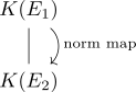
Proof. Let $ϕ : E \to E$ be the $q$ power Frobenius map. By Corollary 7.3

# E (𝔽_{q}) = q + 1 - tr (ϕ) .

Hence $tr (ϕ) = a$ , $\deg (ϕ) = q$ .

Example Sheet 2, Q6(iii) implies $ϕ^{2} - a ϕ = q = 0$ , hence $ϕ^{n = 2} - a ϕ^{n + 1} + q ϕ^{n} = 0$ , so

tr (ϕ^{n + 2}) - a tr (ϕ^{n + 1}) + q tr (ϕ^{n}) = 0 .

This second order difference equation with initial conditions $tr (1) = 2$ , $tr (ϕ) = a$ has solution

tr (ϕ^{n}) = α^{n} + β^{n},

where $α, β$ are roots of $X^{2} - a X + q = 0$ .

Again by Corollary 7.3,

\begin{array}{l} # E (𝔽_{q}^{n}) & = q^{n} + 1 - tr (ϕ^{n}) \\ = 1 + q^{n} - α^{n} - β^{n} \end{array}

Therefore

\begin{array}{l} Z_{E} (T) & = \exp \sum_{n = 1}^{\infty} (\frac{T^{n}}{n} + \frac{{(q T)}^{n}}{n} - \frac{{(α T)}^{n}}{n} - \frac{{(β T)}^{n}}{n}) \\ = \frac{(1 - α T) (1 - β T)}{(1 - T) (1 - q T)} \\ = \frac{1 - a T + q T^{2}}{(1 - T) (1 - q T)} □ \end{array}

Remark. Hasse’s Theorem tells us that $| a | \leq 2 \sqrt{q}$ . $α = \bar{β}$ , and so $| α | = | β | = \sqrt{q}$ $(*)$ .

Let $K = 𝔽_{q} (E)$ . $ζ_{K} (s) = 0$ , so $Z_{E} (q^{- s}) = 0$ , so $q^{s} = α$ or $β$ . Then $q^{Re (s)} = | α |$ or $| β |$ , so by $(*)$ , $Re (s) = \frac{1}{2}$ .

“This is an analog of the Riemann hypothesis.”

8 Formal Groups

Definition ( $I$ -adic topology). Let $R$ be a ring and $I \subset R$ an ideal. The $I$ -adic topology on $R$ has basis ${r + I^{n} | r \in R, n \geq 1}$ .

Definition (Cauchy sequence). A sequence $(x_{n})$ in $R$ is Cauchy if $\forall k, \exists N$ such that $\forall m, n \geq N$ , $x_{m} - x_{n} \in I^{k}$ .

Definition (Complete). $R$ is complete if

(i) $⋂_{n \geq 0} I^{n} = {0}$
(ii) every Cauchy sequence converges

Useful remark: if $x \in I$ then

\frac{1}{1 - x} = 1 + x + x^{2} + \dots

so $1 - x \in R^{\times}$ .

Example. $R = ℤ_{p}$ , $I = p ℤ_{p}$ .

$R = ℤ [[t]]$ , $I = (t)$ .

Lemma 8.1 (Hensel’s Lemma). Assuming that:

$R$ is complete with respect to an ideal $I$
$F \in R [X]$ , $s \geq 1$
$a \in R$ satisfies $F (a) \equiv 0 (m o d I^{s})$ , $F^{'} (a) \in R^{\times}$

Then there exists a unique

b \in R

such that

F (b) = 0

and

b \equiv 0 (m o d I^{s})

Proof. Let $u \in R^{\times}$ with $F (a) = u (m o d I)$ (e.g. we could take $u = F^{'} (a)$ ). Replacing $F (X)$ by $\frac{F (X + a)}{u}$ , we may assume $a = 0$ , $F^{'} (0) \equiv 1 (m o d I)$ .

We put $x_{0} = 0$ ,

x_{n + 1} = x_{n} - F (x_{n}) (1)

Easy induction gives

x_{n} \equiv 0 (m o d I^{s}) \forall n (2)

Let

F (X) - F (Y) = (X - Y) (F^{'} (0) + X G (X, Y) + Y H (X, Y)) (3)

for some $G, H \in R [X, Y]$ .

Claim: $x_{n + 1} \equiv x_{n} (m o d I^{n + s})$ for all $n \geq 0$ .

Proof: By induction on $n$ . Case $n = 0$ is true.

Suppose $x_{n} \equiv x_{n = 1} (m o d I^{n + s - 1})$ . Then

F (x_{n}) - F (x_{n - 1}) = (x_{n} - x_{n - 1}) (1 + c) (m o d I^{n + s})

for some $c \in I$ . Hence

F (x_{n}) - F (x_{n - 1}) = x_{n} - x_{n - 1} (m o d I^{n + s})

Hence

x_{n} - F (x_{n}) \equiv x_{n - 1} - F (x_{n - 1}) (m o d I^{n + s})

and hence $x_{n + 1} \equiv x_{n} (m o d I^{n + s})$ .

This proves the claim.

Therefore ${(x_{n})}_{n \geq 0}$ is Cauchy. Since $R$ is complete, we have $x_{n} \to b$ as $n \to \infty$ for some $b \in R$ .

Taking limit $n \to \infty$ in (1) gives $b = b - F (b)$ , hence $F (b) = 0$ .

Taking limit $n \to \infty$ in (2) gives $b \equiv 0 (m o d I^{s})$ .

Uniqueness is proved using (3) and the “useful remark” (if $x \in I$ then $1 - x \in R^{\times}$ ). □

E : Y^{2} Z + a_{1} X Y Z + a_{3} Y Z^{2} = X^{3} + a_{2} X^{2} Z + a_{4} X Z^{2} + a_{6} Z^{3} .

Affine piece $Y \neq 0$ . $t = - \frac{X}{Y}$ , $w = - \frac{Z}{Y}$ .

w = \underset{= f (t, w)}{\underset{⏟}{t^{3} + a_{1} t w + a_{2} t^{2} w + a_{3} w^{2} + a_{4} t w^{2} + a_{6} w^{3}}} .

We apply Lemma 8.1 with

\begin{array}{l} R & = ℤ [a_{1}, \dots, a_{6}] [[t]] \\ I & = (t) \\ F (X) & = X - f (t, X) \in R [X] \end{array}

$s = 3$ , $a = 0$ .

Check:

\begin{array}{l} F (0) & = - f (t, 0) = - t^{3} \equiv 0 (m o d I^{3}) \\ F^{'} (0) & = 1 - a_{1} t - a_{2} t^{2} \in R^{\times} \end{array}

Hence there exists a unique $w (t) \in R = ℤ [a_{1}, \dots, a_{6}] [[t]]$ such that

\begin{array}{l} w (t) & = f (t, w (t)) \\ w (t) & \equiv 0 (m o d t^{3}) \end{array}

Remark. Taking $u = 1$ in the proof of Lemma 8.1, $w (t) = \lim_{n \to \infty} w_{n} (t)$ where $w_{0} (t) = 0$ , $w_{n + 1} (t) = f (t, w_{n} (t))$ .

In fact,

w (t) = t^{3} (1 + A_{1} t + A_{2} t^{2} + \dots)

where $A_{1} = a_{1}$ , $A_{2} = a_{1}^{2} + a_{2}$ , $A_{3} = a_{1}^{3} + 2 a_{1} a_{2} + 2 a_{3}$ , …

Lemma 8.2. Assuming that:

$R$ an integral domain which is complete with respect to an ideal $I$
$a_{1}, \dots, a_{6} \in R$
$K = Frac (R)$

Then

Ê (I) : = {(t, w) \in E (K) | t, w \in I}

is a subgroup of $E (K)$ .

Note. By uniqueness in Hensel’s lemma:

Ê (I) = {(t, w (t)) \in E (K) | t \in I} .

Proof. Taking $(t, w) = (0, 0)$ show $0_{E} \in Ê (I)$ .

So it suffices to show that $P_{1}, P_{2} \in Ê (I)$ then

\underset{= P_{3}}{\underset{⏟}{- P_{1} - P_{2}}} \in Ê (I) .

$P_{1}, P_{2} \in Ê (I)$ implies $t_{1}, t_{2} \in I$ , $w_{1} = w (t_{1}) \in I$ , $w_{2} = w (t_{2}) \in I$ .

\begin{array}{l} w (t) & = \sum_{n = 2}^{\infty} A_{n - 2} t^{n + 1} & (A_{0} = 1) \\ λ & = {\begin{matrix} \frac{w (t_{2}) - w (t_{1})}{t_{2} - t_{1}} & t_{1} \neq t_{2} \\ w^{'} (t_{1}) & t_{1} = t_{2} \end{matrix} \\ = \sum_{n = 2}^{\infty} A_{n - 2} (t_{1}^{n} + t_{1}^{n - 1} t_{2} + \dots + t_{2}^{n}) \in I \\ ν & = w_{1} - λ t_{1} \in I \end{array}

Substituting $w = λ t + ν$ into $w = f (t, w)$ gives

\begin{array}{l} λ t + ν & = t^{3} + a_{1} t (λ t + ν) + a_{2} t^{2} (λ t + ν) + a_{3} {(λ t + ν)}^{2} + a_{4} t {(λ t + ν)}^{2} + a_{6} {(λ t + ν)}^{3} \\ A & = (coefficient of t^{3}) = 1 + a_{2} λ + a_{4} λ^{2} + a_{6} λ^{3} \\ B & = (coefficient of t^{2}) = a_{1} λ + a_{2} ν + a_{3} λ^{2} + 2 a_{4} λ ν + 3 a_{6} λ^{2} ν \end{array}

We have $A \in R^{\times}$ and $B \in I$ . Hence $t_{3} = - \frac{B}{A} - t_{1} - t_{2} \in I$ , $w_{3} = λ t_{3} + ν \in I$ . □

Taking $R = ℤ [a_{1}, \dots, a_{6}] [[t]]$ , $I = (t)$ , then Lemma 8.2 gives that there exists $ι \in ℤ [a_{1}, \dots, a_{6}] [[t]]$ with $ι (0) = 0$ and

[- 1] (t, w (t)) = (ι (t), w (ι (t))) .

Taking $R = ℤ [a_{1}, \dots, a_{6}] [[t_{1}, t_{2}]]$ , $I = (t_{1}, t_{2})$ , Lemma 8.2 gives that there exists $F \in ℤ [a_{1}, \dots, a_{6}] [[t_{1}, t_{2}]]$ with $F (0, 0) = 0$ and

(t_{1}, w (t_{1})) + (t_{2}, w (t_{2})) = (F (t_{1}, t_{2}), w (F (t_{1}, t_{2})))

and

F (X, Y) = X + Y - a_{1} X Y - a_{2} (X^{2} Y + X Y^{2}) + \dots

By properties of the group law, we deduce

(i) $F (X, Y) = F (Y, X)$
(ii) $F (X, 0) = X$ and $F (0, Y) = Y$
(iii) $F (X, F (Y, Z)) = F (F (X, Y), Z)$
(iv) $F (X, ι (X)) = 0$

Definition (Formal group). Let $R$ be a ring. A formal group over $R$ is a power series $F (X, Y) \in R [[X, Y]]$ satisfying

(i)
$F (X, Y) = F (Y, X)$
(ii)
$F (X, 0) = X$ and $F (0, Y) = Y$
(iii)
$F (X, F (Y, Z)) = F (F (X, Y), Z)$

This looks like it would only define a monoid, but in fact inverses are guaranteed to exist in this context.

Exercise: Show that for any formal group, there exists a unique

ι (X) = - X + \dots \in R [[X]]

such that $F (X, ι (X)) = 0$ .

Example.

(i) $F (X, Y) = X + Y$ (called ${\hat{𝔾}}_{a}$ )
(ii) $F (X, Y) = X + Y + X Y = (1 + X) (1 + Y) - 1$ (called ${\hat{𝔾}}_{m}$ )
(iii) $F (X, Y) = [as above]$ (called $Ê$ )

Definition (Morphism / isomorphic (formal groups)). Let $F$ and $G$ be formal groups over $R$ given by power series $F$ and $G$ .

(i)
A morphism $f : F \to G$ is a power series $f \in R [[T]]$ such that $f (0) = 0$ satisfying
$f (F (X, Y)) = G (f (x), f (Y)) .$
(ii)
$F ≅ G$ if there exists $F \overset{f}{\to} G$ and $G \overset{g}{\to} F$ morphisms such that $f (g (X)) = g (f (X)) = X$ .

Theorem 8.3 (All formal groups are isomorphic). Assuming that:

$char R = 0$

Then any formal group

F

over

R

is isomorphic to

{\hat{𝔾}}_{a}

over

R \otimes ℚ

. More precisely

(i)
There is a unique power series
$\log (T) = T + \frac{a_{2}}{2} T^{2} + \frac{a_{3}}{3} T^{3} + \dots$

with $a_{i} \in R$ such that
$\log (F (X, Y)) = \log (X) + \log (Y) . (∗)$

(ii)

There is a unique power series

\exp (T) = T + \frac{b_{2}}{2!} + \frac{b_{3}}{3!} T^{3} + \dots

with $b_{i} \in R$ such that

\exp (\log (T)) = \log (\exp (T)) = T .

Proof.

(i) Notation

F_{1} (X, Y) = \frac{\partial F}{\partial x} (X, Y)

Uniqueness: Let

p (T) = \frac{d}{d T} \log (T) = 1 + a - 2 T + a_{3} T^{2} + \dots .

Differentiating ( $*$ ) with respect to $X$ gives

p (F (X, Y)) F_{1} (X, Y) = p (X) + 0 .

Putting $X = 0$ gives $p (Y) F_{1} (0, Y) = 1$ , hence $p (Y) = F_{1} {(0, Y)}^{- 1}$ , so $p$ is uniquely determined by $F$ and hence $\log$ is too.

Existence: Let

p (T) = F_{1} {(0, T)}^{- 1} = 1 = a_{2} T + a_{3} T^{2} + \dots

(say). Let

\log (T) = T + \frac{a_{2}}{2} T^{2} + \frac{a_{3}}{3} T^{3} + \dots .

Calculate

\begin{array}{l} F (F (X, Y), Z) & = F (X, F (Y, Z)) \\ F_{1} (F (X, Y), Z) F_{1} (X, Y) & = F_{1} (X, F (Y, Z)) & \frac{d}{d x} \\ F_{1} (Y, Z) F_{1} (0, Y) & = F_{1} (0, F (Y, Z)) & put X = 0 \\ ⟹ F_{1} (Y, Z) p {(Y)}^{- 1} & = p {(F (Y, Z))}^{- 1} \\ ⟹ F_{1} (Y, Z) p (F (Y, Z)) & = p (Y) \\ \log (F (Y, Z)) & = \log (Y) + h (Z) & integrate w.r.t. Y \end{array}

for some power series $h$ .

Symmetry $Y \leftrightarrow Z$ gives $h (Z) = \log (Z)$ .

This proves existence.

(ii) We prove a lemma first. □

Lemma 8.4. Assuming that:

$f (T) = a T + \dots \in R [[T]]$ with $a \in R^{\times}$

Then there exists a unique

g (T) = a^{- 1} T + \dots \in R [[T]]

such that

f (g (T)) = g (f (T)) = T

Proof. We construct polynomials $g_{n} (T) \in R [T]$ such that

\begin{array}{l} f (g_{n} (T)) & \equiv T (m o d T^{n + 1}) \\ g_{n + 1} (T) & \equiv g_{n} (T) (m o d T^{n + 1}) \end{array}

Then $g (T) = \lim_{n \to \infty} g_{n} (T)$ satisfies $f (g (T)) = T$ .

To start the induction, we set $g_{1} (T) = a^{- 1} T$ . Now suppose $n \geq 2$ and $g_{n - 1} (T)$ exists. Then

f (g_{n - 1} (T)) \equiv T + b T^{n} (m o d T^{n + 1}) .

We put $g_{n} (T) = g_{n - 1} (T) + λ T^{n}$ for some $λ \in R$ to be chosen later.

Then

\begin{array}{l} f (g_{n} (T)) & = f (g_{n - 1} (T) + λ T^{n}) \\ \equiv f (g_{n - 1} (T)) + λ a T^{n} (m o d T^{n + 1}) \\ \equiv T + (b + λ a) T^{n} (m o d T^{n + 1}) \end{array}

We take $λ = - \frac{b}{a}$ ( $a \in R^{\times}, b \in R ⟹ λ \in R$ ).

This completes the induction step.

We get $g (T) = a^{- 1} T + \dots \in R [[T]]$ such that $f (g (T)) = T$ . Applying the same construction to $g$ gives $h (T) = a T + \dots \in R [[T]]$ such that $g (h (T)) = T$ .

Now note $f (T) = f (g (h (T))) = h (T)$ . □

Theorem 8.3(ii) now follows by Lemma 8.4 and Q12 from Example Sheet 2.

Notation. Let $F$ (e.g. ${\hat{𝔾}}_{a}$ , ${\hat{𝔾}}_{m}$ , $Ê$ ) be a formal group given by a power series $F \in R [[X, Y]]$ .

Suppose $R$ is a ring complete with respect to ideal $I$ . For $x, y \in I$ , put

x \oplus_{F} y = F (x, y) \in I .

Then $F (I) : = (I, \oplus_{F})$ is an abelian group.

Examples:

${\hat{𝔾}}_{a} (I) = (I, +)$
${\hat{𝔾}}_{m} (I) = (1 + I, \times)$
$Ê (I) = subgroup of E (K) in Lemma 8.2$

Corollary 8.5. Assuming that:

$F$ a formal group over $R$
$n \in ℤ$ such that $n \in R^{\times}$

Then

(i) $[n] : F \to F$ is an isomorphism of formal groups
(ii) If $R$ is complete with respect to ideal $I$ then $F (I) \overset{\times n}{\to} F (I)$ is an isomorphism of groups. In particular, $F (I)$ has no $n$ -torsion.

Proof. We have

\begin{array}{l} [1] (T) & = T \\ [n] (T) & = F ([n - 1] (T), T) \end{array}

(for $n < 0$ use $[- 1] (T) = ι (T)$ ).

Since

F (X, Y) = X + Y + X Y (\dots)

we get

[2] (T) = F (T, T) 2 T + \dots \in R [[T]]

and by induction we get

[n] (T) = n T + \dots \in R [[T]] .

Lemma 8.4 shows that if $n \in R^{\times}$ then $[n]$ is an isomorphism. This proves (i), and (ii) follows. □

9 Elliptic Curves over Local Fields

Let $K$ be a field, complete with respect to discrete valuation $v : K^{*} \to ℤ$ .

Notation. Valuation ring (= ring of integers) will be denoted by

O_{K} = {x \in K^{*} | v (x) \geq 0} \cup {0} .

Unit group will be denoted by

O_{K}^{*} = {x \in K^{*} | v (x) = 0} .

The maximal ideal will be denoted by $π O_{K}$ where $v (π) = 1$ .

The residue field will be denoted by $k = O_{K} ∕ π O_{K}$ .

We assume $char K = 0$ and $char k = p > 0$ . For example, $K = ℚ_{p}$ , $O_{K} = ℤ_{p}$ , $k = 𝔽_{p}$ .

Let $E ∕ K$ be an elliptic curve.

Definition (Integral / minimal Weierstrass equation). A Weierstrass equation for $E$ with coefficients $a_{1}, \dots, a_{6} \in K$ is integral if $a_{1}, \dots, a_{6} \in O_{K}$ and minimal if $v (Δ)$ is minimal among all integral Weierstrass equations for $E$ .

Remark.

(i) Putting $x = u^{2} x^{'}$ , $y = u^{3} y^{'}$ gives $a_{i} = u^{i} a_{i}^{'}$ . Therefore integral Weierstrass equations exist.
(ii) $a_{1}, \dots, a_{6} \in O_{K} ⟹ Δ \in O_{K} ⟹ v (Δ) \geq 0$ . Therefore minimal Weierstrass equations exist.
(iii) If $char k \neq 2, 3$ then there exists minimal Weierstrass equation of the form $y^{2} = x^{3} + a x + b$ .

Lemma 9.1. Assuming that:

E ∕ K

have integral Weierstrass equation

y^{2} + a_{1} x y + a_{3} y = x^{3} + a_{2} x^{2} + a_{4} x + a_{6}

$0 \neq P = (x, y) \in E (K)$

Then either

x, y \in O_{K}

{\begin{matrix} v (x) = - 2 s \\ v (y) = - 3 s \end{matrix}

for some $s \geq 1$ .

(Compare with Q5 from Example Sheet 1)

Proof. Throughout this proof, LHS and RHS refer to the Weierstrass equation of the curve.

Case $v (x) \geq 0$ :. If $v (y) < 0$ then $v (LHS) < 0$ and $v (RHS) \geq 0$ . Therefore $x, y \in O_{K}$ .

Case $v (x) < 0$ : $v (LHS) \geq \min (2 v (y), v (x) + v (y), v (y))$ and $v (RHS) = 3 v (x)$ . We get 3 possible inequalities from this, and each of them gives $v (y) < v (x)$ .

Now

\begin{array}{l} v (LHS) & = 2 v (y) \\ v (RHS) & = 3 v (x) \end{array}

{\begin{matrix} v (x) = - 2 s \\ v (y) = - 3 s \end{matrix}

for some $s \geq 1$ . □

If $K$ is complete, then $O_{K}$ is complete with respect to $π^{r} O_{K}$ (for any $r \geq 1$ ).

We fix a minimal Weierstrass equation for $E ∕ K$ . Get formal group $Ê$ over $O_{K}$ .

Taking $I = π^{r} O_{K}$ (with $r \geq 1$ ) in Lemma 8.2 gives

\begin{array}{l} Ê (I) & = {(x, y) \in E (K) | - \frac{x}{y}, - \frac{1}{y} \in π^{r} O_{K}} \cup {0} \\ = {(x, y) \in E (K) | v (\frac{x}{y}) \geq r, v (\frac{1}{y}) \geq r} \cup {0} \\ = {(x, y) \in E (K) | v (x) = - 2 s, v (y) = - 3 s for s \geq r} \cup {0} & (using Lemma 9.1) \\ = {(x, y) \in E (K) | v (x) \leq - 2 r, v (y) \leq - 3 r} \cup {0} & (using Lemma 9.1) \end{array}

By Lemma 8.2 this is a subgroup of $E (K)$ , say $E_{r} (K)$ .

\dots \subset E_{2} (K) \subset E_{1} (K) \subset E (K) .

More generally, for $F$ a formal group over $O_{K}$

\dots \subset F (π^{2} O_{K}) \subset F (π O_{K}) .

We claim that

$F (π^{r} O_{K}) ≅ (O_{K}, +)$ for $r$ sufficiently large.
$\frac{F (π^{r} O_{K})}{F (π^{r + 1} O_{K})} ≅ (k, +)$ for $r \geq 1$ .

Reminder: $char K = 0$ , $char k = p > 0$ .

Theorem 9.2. Assuming that:

$K$ a local field with $char K = 0$ , $char k = p > 0$
$F$ a formal group over $O_{K}$
$e = v (p)$
$r > \frac{e}{p - 1}$

Then

\log : F (π^{r} O_{K}) \to_{}^{≅} {\hat{𝔾}}_{a} (π^{r} O_{K})

is an isomorphism of groups with inverse

\exp : {\hat{𝔾}}_{a} (π^{r} O_{K}) \to_{}^{≅} F (π^{r} O_{K}) .

Remark. ${\hat{𝔾}}_{a} (π^{r} O_{K}) = (π^{r} O_{K}, +) ≅ (O_{K}, +)$ , $x \leftrightarrow π^{- r} x$ .

Proof. For $x \in π^{r} O_{K}$ we must show the power series $\log (x)$ and $\exp (x)$ converge to elements in $π^{r} O_{K}$ .

Recall

\exp (T) = T + \frac{b_{2}}{2!} T^{2} + \frac{b_{3}}{3!} T^{3} + \dots

for some $b_{i} \in O_{K}$ .

Claim: $v_{p} (n!) \leq \frac{n - 1}{p - 1}$ .

Proof of claim:

v_{p} (n!) = \sum_{r = 1}^{\infty} ⌊ \frac{n}{p^{r}} ⌋ < \sum_{r = 1}^{\infty} \frac{n}{p^{r}} = \frac{n \cdot \frac{1}{p}}{1 - \frac{1}{p}} = \frac{n}{p - 1} .

Therefore

\begin{array}{l} (p - 1) v_{p} (n!) & < n \\ (p - 1) v_{p} (n!) & \leq n - 1 \end{array}

(we go from $<$ to $\leq ∙ - 1$ by noting that the LHS is in $ℤ$ ).

This proves the claim.

Now

\begin{array}{l} v (\frac{b_{n} x^{n}}{n!}) & \geq n r - e (\frac{n - 1}{p - 1}) \\ = (n - 1) \underset{> 0}{\underset{⏟}{(r - \frac{e}{p - 1})}} + r \end{array}

This is always $\geq r$ and $\to \infty$ as $n \to \infty$ . Therefore $\exp (x)$ converges to an element in $π^{r} O_{K}$ .

Same method works for $\log$ . □

Lemma 9.3. $\frac{F (π^{r} O_{K})}{F (π^{r + 1} O_{K})} ≅$ $(k, +)$ for all $r \geq 1$ .

Proof. Definition of formal group gives

F (X, Y) = X + Y + X Y (\dots) .

So if $x, y \in O_{K}$ ,

F (π^{r} x, π^{r} y) \equiv π^{r} (x + y) (m o d π^{r + 1}) .

Therefore

\begin{array}{l} F (π^{r} O_{K}) & \to (k, +) \\ π^{r} x & \mapsto x mod π \end{array}

is a surjective group homomorphism with kernel $F (π^{r + 1} O_{K})$ . □

Corollary. Assuming that:

$| k | < \infty$

Then

F (π O_{K})

has a subgroup of finite index isomorphic to

(O_{K}, +)

Notation. Reduction modulo $π$

\begin{array}{l} O_{K} & \to \frac{O_{K}}{π O_{K}} = k \\ x & \mapsto \tilde{x} \end{array}

Proposition 9.4. Assuming that:

$E ∕ K$ be an elliptic curve

Then the reduction mod

π

of any two minimal Weierstrass equations for

E

define isomorphic curves over

k

Proof. Say Weierstrass equations are related by $[u; r, s, t]$ , $u \in K^{*}$ , $r, s, t \in K$ . Then $Δ_{1} = u^{12} Δ_{2}$ . Both equations minimal gives us that $v (Δ_{1}) = v (Δ_{2})$ , hence $u \in O_{K}^{*}$ .

Transformation formula for the $a_{i}$ and $b_{i} + O_{K}$ is integrally closed, hence $r, s, t \in O_{K}$ .

The Weierstrass equations obtained by reducing mod $π$ are now related by $[ũ; \tilde{r}, \tilde{s}, \tilde{t}]$ , $ũ \in k^{*}$ , $\tilde{r}, \tilde{s}, \tilde{t} \in k$ . □

Definition. The reduction $Ẽ ∕ k$ of $E ∕ K$ is defined by the reduction of a minimal Weierstrass equation.

$E$ has good reduction if $Ẽ$ is non-singular (and so an elliptic curve) otherwise has bad reduction.

For an integral Weierstrass equation,

If $v (Δ) = 0$ then good reduction.
If $0 < v (Δ) < 12$ then bad reduction.
If $v (Δ) \geq 12$ then beware that the equation might not be minimal.

There is a well-defined map

\begin{array}{l} ℙ^{2} (K) & \to ℙ^{2} (k) \\ (x : y : z) & \mapsto (\tilde{x} : ỹ : \tilde{z}) \end{array}

(choose a representative with $\min (v (x), v (y), v (z)) = 0$ ).

We restrict to give

\begin{array}{l} E (K) & \to Ẽ (K) \\ P & \mapsto \tilde{P} \end{array}

If $P = (x, y) \in E (K)$ then by Lemma 9.1 either

$x, y \in O_{K}$ in which case $\tilde{P} = (\tilde{x}, ỹ)$ .
or $v (x) = - 2 s$ , $v (y) = - 3 s$ for some $s \geq 1$ , in which case $P = (x : y : 1) = (π^{3 s} x : π^{3 s} y : π^{3 s})$ and $\tilde{P} = (0 : 1 : 0)$ .

Therefore

E_{1} (K) = I d i d n^{'} t m a n a g e t o w r i t e t h i s b e f o r e i t w a s r u b b e d o f f

“kernel of reduction”.

Notation.

{\begin{matrix} Ẽ & if E has good reduction \\ Ẽ ∖ {singular point} & if E has bad reduction \end{matrix}

The chord and tangent process still defines a group law on $Ẽ_{ns}$ .

In cases of bad reduction, $Ẽ_{ns} ≅ 𝔾_{m}$ (over $k$ or possibly a quadratic extension of $k$ ) or $Ẽ_{ns} ≅ 𝔾_{a}$ (over $k$ ).

For simplicity we suppose $char k \neq 2$ .

Then $Ẽ = y^{2} = f (x)$ , $\deg f = 3$ .

\begin{array}{l} Ẽ_{ns} & \to_{}^{≅} 𝔾_{a} \\ (x, y) & \mapsto \frac{x}{y} \\ (t^{- 2}, t^{- 3}) & \leftarrow ↤ t \\ (point at \infty) & \leftarrow ↤ 0 \end{array}

Let

P_{1}, P_{2}, P_{3}

lie on the line

a x + b y = 1

. Write

P_{i} = (x_{i}, y_{i})

t_{i} = \frac{x_{i}}{y_{i}}

. Then

x_{i}^{3} = y_{i}^{2} = y_{i}^{2} (a x_{i} + b y_{i})

. So

t_{i}^{3} - a t_{i} - b = 0

. So

t_{1}, t_{2}, t_{3}

are the roots of

T^{3} - a T - b = 0

Looking at coefficient of $T^{2}$ gives $t_{1} + t_{2} + t_{3} = 0$ .

Definition ( $E_{0} (K)$ ). $E_{0} (K) = {P \in E (K) | \tilde{P} \in Ẽ_{ns} (k)}$ .

Proposition 9.5. $E_{0} (K)$ is a subgroup of $E (K)$ and reduction modulo $π$ is a surjective group homomorphism $E_{0} (K) \to Ẽ_{ns} (k)$ .

Note. If $E ∕ K$ has good reduction, then this is a surjective group homomorphism $E (K) \to Ẽ (k)$ .

Proof. Group homomorphism: A line $l$ in $ℙ^{2}$ defined over $K$ has equation

l : a X + b Y + c Z = 0 a, b, c \in K .

We may assume $\min (v (a), v (b), v (c)) = 0$ . Reduction modulo $π$ gives a line

\tilde{l} : ã X + \tilde{b} Y + \tilde{c} Z = 0 .

If $P_{1}, P_{2}, P_{3} \in E (K)$ with $P_{1} + P_{2} + P_{3} = 0$ then these points lie on a line $l$ . So ${\tilde{P}}_{1}, {\tilde{P}}_{2}, {\tilde{P}}_{3}$ lie on the line $\tilde{l}$ . If ${\tilde{P}}_{1}, {\tilde{P}}_{2} \in {\tilde{(}}_{ns} k)$ then ${\tilde{P}}_{3} \in {\tilde{(}}_{ns} k)$ .

So if $P_{1}, P_{2} \in E_{0} (K)$ then $P_{3} \in E_{0} (K)$ and ${\tilde{P}}_{1} + {\tilde{P}}_{2} + {\tilde{P}}_{3} = 0$ .

[Exercise: check this still works if $# {{\tilde{P}}_{1}, {\tilde{P}}_{2}, {\tilde{P}}_{3}} < \infty$ ]

Surjective: Let $f (x, y) = y^{2} + a_{1} x y + a_{3} y - (x^{3} + \dots)$ . Let $\tilde{P} \in Ẽ_{ns} (k) ∖ {0}$ , say $\tilde{P} = ({\tilde{x}}_{0}, ỹ_{0})$ for some $x_{0}, y_{0} \in O_{K}$ .

Since $\tilde{P}$ non-singular, either:

(i) $\frac{\partial f}{\partial x} (x_{0}, y_{0}) ⁄ \equiv 0 (m o d π)$ .
(ii) $\frac{\partial f}{\partial y} (x_{0}, y_{0}) ⁄ \equiv 0 (m o d π)$ .

If (i) then put $g (t) = f (t, y_{0}) \in O_{K} [t]$ . Then

{\begin{matrix} g (x_{0}) \equiv 0 & (m o d π) \\ g^{'} (x_{0}) \in O_{K}^{*} \end{matrix}

Hensel’s lemma gives us that there exists $b \in O_{K}$ such that

{\begin{matrix} g (b) = 0 \\ b \equiv x_{0} (m o d π) \end{matrix}

Then $(b, y_{0}) \in E (K)$ has erduction $\tilde{P}$ . asdfadsf □

Recall that for $r \geq 1$ we put

E_{r} (K) = {(x, y) | v (x) \leq - 2 r, v (y) \leq - 3 r} \cup {0} .

If $r > \frac{e}{p - 1}$ , these give:

\underset{≅ (O_{K}, +)}{\underset{⏟}{E_{r} (K)}} \subset \dots \subset \underset{= Ê (π^{2} O_{K})}{\underset{⏟}{E_{2} (K)}} \subset \underset{= Ê (π O_{K})}{\underset{⏟}{E_{1} (K)}} \subset E_{0} (K) \subset E (K),

where for $i \geq 1$ , each $E_{i + 1} (K) \subset E_{i} (K)$ gives a quotient isomorphic to $(k, +)$ .

We have $\frac{E_{0} (K)}{E_{1} (K)} ≅ Ẽ_{ns} (k)$ .

What about $\frac{E (K)}{E_{0} (K)}$ ?

Lemma 9.6. Assuming that:

$| k | < \infty$

Then

E_{0} (K) \subset E (K)

has finite index.

Proof. $| k | < \infty$ implies that $\frac{O_{K}}{π^{r} O_{K}}$ is finite for all $r \geq 1$ .

Hence

O_{K} ≅ \lim_{\overset{[}{r}] \leftarrow} \frac{O_{K}}{π^{r} O_{K}}

is a profinite group, hence compact.

Then $ℙ^{n} (K)$ is the union of sets

{(a_{0} : \dots : a_{i - 1} : 1 : a_{i + 1} : \dots : a_{n}) : a_{j} \in O_{K}}

and hence compact (for the $π$ -adic topology).

Now note $E (K) \subset ℙ^{2} (K)$ is a closed subset, hence compact.

So $E (K)$ is a compact topological group.

If $Ẽ$ has a singular point $({\tilde{x}}_{0}, ỹ_{0})$ then

E (K) ∖ E_{0} (K) = {(x, y) \in E (K) | v (x - x_{0}) \geq 1, v (y - y_{0}) \geq 1}

is a closed subset of $E (K)$ hence $E_{0} (K)$ is an open subgroup of $E (K)$ .

The cosets of $E_{0} (K)$ are an open cover of $E (K)$ . Hence $[E (K) : E_{0} (K)] < \infty$ . □

Definition (Tamagawa number). $c_{K} (E) = [E (K) : E_{0} (K)]$ is called the Tamagawa number.

Remark.

(i) If we have good reduction then $c_{K} (E) = 1$ (converse is false).
(ii) It can be shown that
- either $c_{K} (E) = v (Δ)$
- or $c_{K} (E) \leq 4$
for the above statements: it is essential that we work with minimal Weierstrass equations.

We deduce:

Theorem 9.7. Assuming that:

$[K : ℚ_{p}] < \infty$

Then

E (K)

contains a subgroup of finite index isomorphic to

(O_{K}, +)

Let $[K : ℚ_{p}] < \infty$ and $L ∕ K$ a finite extension. Let the residue fields be $k^{'}$ and $k$ , and let $f = [k^{'} : k]$ .

Facts:

(i) $[L : K] = e f$ .
(ii) If $L ∕ K$ is Galois then the natural map $Gal (L ∕ K) \to Gal (k^{'} ∕ k)$ is surjective with kernel of order $e$ .

Definition (Unramified). $L ∕ K$ is unramified if $e = 1$ .

Fact: For each $m \geq 1$

(i) $k$ has a unique extension of degree $m$ (say $k_{m}$ ).
(ii) $K$ has a unique unramified extension of degree $m$ (say $K_{m}$ ).

These extensions are Galois, with cyclic Galois groups.

Definition (Maximal unramified extension). $K^{nr} = ⋃_{m \geq 1} K_{m}$ (inside $\bar{K}$ ). “maximal unramified extension”

Theorem 9.8. Assuming that:

$[K : ℚ_{p}] < \infty$
$E ∕ K$ has good reduction
$p ∤ n$
$P \in E (K)$

Then

K ({[n]}^{- 1} P) ∕ K

is unramified.

Notation.

{[n]}^{- 1} (P) = {Q \in E (\bar{K}) : n Q = P},

K ({Q_{1}, \dots, Q_{r}}) = K (x_{1}, \dots, x_{r}, y_{1}, \dots, y_{r}),

where $Q_{i} = (x_{i}, y_{i})$ .

Proof. For each $m \geq 1$ there is a short exact sequence

0 \to E_{1} (K_{m}) \to E (K_{m}) \to Ẽ (K_{m}) \to 0 .

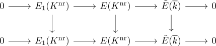
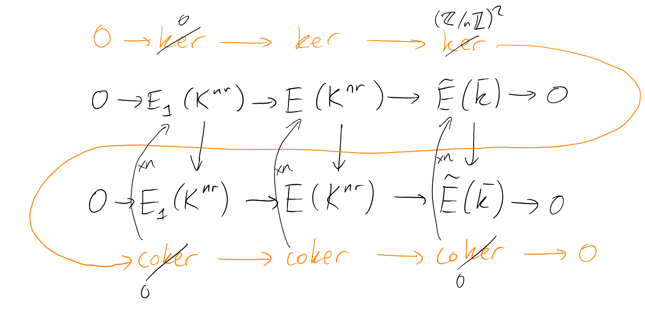
Taking $⋃_{m \geq 1}$ gives a commutative diagram with exact rows:

--
0 E1(Knr) E (Knr) ˜E(k) 0

0 E1(Knr) E (Knr) ˜E(k) 0

An isomorphism by Corollary 8.5 applied over each $K_{m}$ (using $p ∤ n$ here).

surjective by Theorem 2.8
kernel $≅ {(ℤ ∕ n ℤ)}^{2}$ by Theorem 6.5 (again using $p ∤ n$ ).

Snake lemma gives

{\begin{matrix} E (K^{nr}) [n] ≅ {(ℤ ∕ n ℤ)}^{2} \\ \frac{E (K^{nr})}{n E (K^{nr})} = 0 \end{matrix}

So if $P \in E (K)$ then there exists $Q \in E (K^{nr})$ such that $n Q = P$ and

{[n]}^{- 1} P = {Q + T : T \in E [n]} \subset E (K^{nr}) .

Hence $K ({[n]}^{- 1} P) \subset K^{nr}$ and so $K ({[n]}^{- 1} P) ∕ K$ is unramified. □

10 Elliptic Curves over Number Fields: The torsion subgroup

$[K : ℚ] < \infty$ , $E ∕ K$ an elliptic curve.

Notation. $𝔭$ a prime of $K$ (i.e. a prime) ideal in $O_{K}$ ).

$K_{𝔭}$ is the $𝔭$ -adic completion of $K$ , valuation ring $O_{𝔭}$ .

$k_{𝔭} = O_{K} ∕ 𝔭$ residue field.

Definition (Good reduction (prime)). $𝔭$ is a prime of good reduction for $E ∕ K$ if $E ∕ K_{𝔭}$ has good reduction.

Lemma 10.1. $E ∕ K$ has only finitely many primes of bad reduction.

Proof. Take a Weierstrass equation for $E$ with $a_{1}, \dots, a_{6} \in O_{K}$ . $E$ non-singular implies that $0 \neq Δ \in O_{K}$ .

Write $(Δ) = 𝔭^{α_{1}} \dots 𝔭_{r}^{α_{r}}$ (factorisation into prime ideals).

Let $S = {𝔭_{1}, \dots, 𝔭_{r}}$ . If $𝔭 \notin S$ then $v_{𝔭} (Δ) = 0$ . Hence $E ∕ K_{𝔭}$ has good reduction.

Therefore ${bad primes for E} \subset S$ , hence is finite. □

Remark. If $K$ has class number $1$ (e.g. $K = ℚ$ ) then we can always find a Weierstrass equation for $E$ with $a_{1}, \dots, a_{6} \in O_{K}$ which is minimal at all primes $𝔭$ .

Basic group theory: If $A$ is a finitely generatead abelian group then $A ≅ {finite group} \times ℤ^{r}$ . We call $r$ the “rank”, and ${finite subgroup}$ is the torsion subgroup.

Lemma 10.2. $E {(K)}_{tors}$ is finite.

Proof. Take any prime $𝔭$ . We saw that $E (K_{𝔭})$ has a finite index subgroup $A$ (say) with $A ≅ (O_{𝔭}, +)$ .

In particular, $A$ is torsion free

E {(K)}_{tors} ↪ E {(K_{𝔭})}_{tors} ↪ \underset{finite}{\underset{⏟}{\frac{E (K_{𝔭})}{A}}} . □

Lemma 10.3. Assuming that:

$𝔭$ is a prime of good reduction
$𝔭 ∤ n$

Then reduction modulo

𝔭

gives an injective group homomorphism

E (K) [n] ↪ Ẽ (k_{𝔭}) .

Proof. Proposition 9.5 gives that $E (K_{𝔭}) \to Ẽ (k_{𝔭})$ is a group homomorphism, with kernel $E_{1} (K_{𝔭})$ .

Corollary 8.5 and $𝔭 ∤ n$ gives that $E_{1} (K_{𝔭})$ has no $n$ -torsion. □

Example. $E ∕ ℚ$ : $y^{2} + y = x^{3} - x$ , $Δ = - 11$ .

$E$ has good reduction at all $p \neq 11$ .

$p$	$2$	$3$	$5$	$7$	$11$	$13$

$# Ẽ (𝔽_{p})$	$5$	$5$	$5$	$5$	$-$	$10$

Lemma 10.3 gives:

{\begin{matrix} # {(ℚ)}_{tors} | 5 \cdot 2^{a} & for some a \geq 0 \\ # E {(ℚ)}_{tors} | 5 \cdot 3^{b} & for some b \geq 0 \end{matrix}

Hence $# {(ℚ)}_{tors} | 5$ .

Let $T = (0, 0) \in E (ℚ)$ . Calculation gives $5 T = 0$ . Therefore $E {(ℚ)}_{tors} ≅ ℤ ∕ 5 ℤ$ .

Example. $E ∕ ℚ$ : $y^{2} + y = x^{3} + x^{2}$ , $Δ = - 43$

$p$	$2$	$3$	$5$	$7$	$11$	$13$

$# Ẽ (𝔽_{p})$	$5$	$6$	$10$	$8$	$9$	$19$

Lemma 10.3 gives:

{\begin{matrix} # E {(ℚ)}_{tors} | 5 \cdot 2^{a} & for some a \geq 0 \\ # E {(ℚ)}_{tors} | 9 \cdot 1 1^{b} & for some b \geq 0 \end{matrix}

Therefore $E {(ℚ)}_{tors} = {0}$ .

Therefore $P = (0, 0)$ is a point of infinite order.

In particular, $E (ℚ)$ is infinite.

Example. $E_{D}$ : $y^{2} = x^{3} - D^{2} x = f (x)$ . $D \in ℤ$ square-free, $Δ = 2^{6} D^{6}$ . If $p ∤ 2 D$ , then

# Ẽ_{D} (𝔽_{p}) = 1 + \sum_{x \in 𝔽_{p}} ((\frac{f (x)}{p}) + 1) .

If $p \equiv 3 (m o d 4)$ then since $f$ is odd,

(\frac{f (- x)}{p}) = (\frac{- f (x)}{p}) = (\frac{- 1}{p}) (\frac{f (x)}{p}) = - (\frac{f (x)}{p}) .

Hence

# Ẽ_{D} (𝔽_{p}) = p + 1 .

E_{D} {(ℚ)}_{tors} \supset {0, (0, 0), (\pm D, 0)} ≅ {(ℤ ∕ 2 ℤ)}^{2} .

Let $m = # E_{D} {(ℚ)}_{tors}$ .

We have $4 | m | p + 1$ forr all sufficiently large ( $p ∤ 2 m D$ ) primes $p$ with $p \equiv 3 (m o d 4)$ . Hence $m = 4$ (otherwise get contradiction to Dirichlet’s theorem on primes on arithmetic progressions).

\begin{array}{l} rank E_{D} (ℚ) \geq 1 & ⟺ \exists x, y \in ℚ, y \neq 0 \land y^{2} = x^{3} - D^{2} x \\ \overset{Lecture 1}{⟺} D is a congruent number \end{array}

Lemma 10.4. Assuming that:

$E ∕ ℚ$ is given by a Weierstrass equation with $a_{1}, \dots, a_{6} \in ℤ$
$0 \neq T = (x, y) \in E {(ℚ)}_{tors}$

Then

(i) $4 x, 8 y \in ℤ$
(ii) If $2 | a_{1}$ or $2 T \neq 0$ then $x, y \in ℤ$

Proof.

(i) The Weierstrass equation defines a formal group $Ê$ over $ℤ$ . For $r \geq 1$ ,
$Ê (p^{r} ℤ_{p}) = {(x, y) \in E (ℚ_{p}) | v_{p} (x) \leq - 2 r, v_{p} (y) \leq - 3 r} \cup {0} .$

Then Theorem 9.2 gives $Ê (p^{r} ℤ_{p}) ≅ (ℤ_{p}, +)$ if $r > \frac{1}{p - 1}$ . Hence $Ê (4 ℤ_{2})$ and $Ê (p ℤ_{p})$ for $p$ are odd are torsion free.

So if $0 \neq T = (x, y) \in E {(ℚ)}_{tors}$ then
$\begin{array}{l} v_{2} (x) & \geq - 2 \\ v_{2} (y) & \geq - 3 \\ v_{p} (x) & \geq 0 \\ v_{p} (y) & \geq 0 \end{array}$
for all odd primes $p$ .

(ii) Suppose

T \in Ê (2 ℤ_{2})

, i.e.

v_{2} (x) = - 2

v_{2} (y) = - 3

Since

\frac{Ê (2 ℤ_{2})}{Ê (4 ℤ_{2})} ≅ (𝔽_{2}, +)

and $Ê (4 ℤ_{2})$ is torsion free, we get $2 T = 0$ .

Also $(x, y) = T = - T = (x, - y - a_{1} x - a_{3})$ . So

\begin{array}{l} 2 y + a_{1} x + a_{3} & = 0 \\ \underset{odd}{\underset{⏟}{8 y}} + a_{1} \underset{odd}{\underset{⏟}{(4 x)}} + \underset{even}{\underset{⏟}{4 a_{3}}} & = 0 \end{array}

Hence $a_{1}$ is odd.

So if $2 T \neq 0$ or $a_{1}$ is even then $T \notin Ê (2 ℤ_{2})$ , so $x, y \in ℤ$ . □

Example. $y^{2} + x y = x^{3} + 4 x + 1$ , $(- \frac{1}{4}, \frac{1}{8}) \in E (ℚ) [2]$ .

Theorem 10.5 (Lutz Nagell). Assuming that:

$E ∕ ℚ$ : $y^{2} = x^{3} + a x + b$ , $a, b \in ℤ$
$0 \neq T = (x, y) \in E {(ℚ)}_{tors}$

Then

x, y \in ℤ

and either

y = 0

y^{2} | (4 a^{3} + 27 b^{2})

Proof. Lemma 10.4 gives that $x, y \in ℤ$ .

If $2 T = 0$ then $y = 0$ . Otherwise $0 \neq 2 T = (x_{2}, y_{2}) \in E {(ℚ)}_{tors}$ .

Lemma 10.4 gives $x_{2}, y_{2} \in ℤ$ . But

x_{2} = {(\frac{f^{'} (x)}{2 y})}^{2} - 2 x

hence $y | f^{'} (x)$ .

$E$ non-singular gives that $f (X)$ adn $f^{'} (X)$ are coprime, so $f (X)$ and $f^{'} {(X)}^{2}$ are coprime. Therefore there exists $g, h \in ℚ [X]$ satisfying

g (X) f (X) + h (X) f^{'} {(X)}^{2} = 1 .

Doing this and clearing denominators gives

(3 X^{2} + 4 a) f^{'} {(X)}^{2} - 27 (X^{3} + a X - b) f (X) = 4 a^{3} + 27 b^{2} .

Since $y | f^{'} (x)$ and $y^{2} = f (x)$ , we get $y^{2} | (4 a^{3} + 27 b^{2})$ . □

Remark. Mazur showed that if $E ∕ ℚ$ is an elliptic curve then

E {(ℚ)}_{tors} ≅ {\begin{matrix} ℤ ∕ n ℤ & 1 \leq n \leq 12, n \neq 11 \\ ℤ ∕ 2 ℤ \times ℤ ∕ 2 n ℤ & 1 \leq n \leq 4 \end{matrix}

Moreover, all 15 possibilities occur.

11 Kummer Theory

Let $K$ be a field and $char K ∤ n$ . Assume $μ_{n} \subset K$ .

Lemma 11.1. Assuming that:

$Δ \subset K^{*} ∕ {(K^{*})}^{n}$ a finite subgroup
$L = K (\sqrt[n]{Δ})$

Then

L ∕ K

is Galois and

Gal (L ∕ K) ≅ Hom (Δ, μ_{n})

Proof. $μ_{n} \subset K$ gives $L ∕ K$ normal, and $char K ∤ n$ gives that $L ∕ K$ is separable. So $L ∕ K$ is Galois.

Define the Kummer pairing

\begin{array}{l} ⟨, ⟩ : Gal (L ∕ K) \times Δ & \to μ_{n} \\ (σ, x) & \mapsto \frac{σ (\sqrt[n]{x})}{\sqrt[n]{x}} \end{array}

Well-defined: Suppose $α, β \in L$ with $α^{n} = β^{n} = x$ . Then ${(\frac{α}{β})}^{n} = 1$ , so $\frac{α}{β} \in μ_{n} \subset K$ . Then $σ (\frac{α}{β}) = \frac{α}{β}$ for all $σ \in Gal (L ∕ K)$ , hence $\frac{σ (α)}{α} = \frac{σ (β)}{β}$ for all $σ \in Gal (L ∕ K)$ .

Bilinear:

\begin{array}{l} ⟨ σ τ, x ⟩ & = \frac{σ (τ \sqrt[n]{x})}{τ \sqrt[n]{x}} \frac{τ \sqrt[n]{x}}{\sqrt[n]{x}} & = ⟨ σ, x ⟩ ⟨ τ, x ⟩ \\ ⟨ σ, x y ⟩ & = \frac{σ \sqrt[n]{x y}}{\sqrt[n]{x y}} \\ = \frac{σ \sqrt[n]{x}}{\sqrt[n]{x}} \frac{σ \sqrt[n]{y}}{\sqrt[n]{y}} \\ = ⟨ σ, x ⟩ ⟨ σ, y ⟩ \end{array}

Non-degenerate: Let $σ \in Gal (L ∕ K)$ . If $⟨ σ, x ⟩ = 1$ for all $x \in Δ$ , then

σ \sqrt[n]{x} = \sqrt[n]{x} \forall x \in Δ

adn hence $σ$ fixes $L$ pointwise, i.e. $σ = 1$ .

Let $x {(K^{*})}^{n} \in Δ$ . If $⟨ σ, x ⟩ = 1$ for all $σ \in Gal (L ∕ K)$ , then

σ \sqrt[n]{x} = \sqrt[n]{x} \forall σ \in Gal (L ∕ K) .

So $\sqrt[n]{x} \in K$ , so $x \in {(K^{*})}^{n}$ , i.e. $x {(K^{*})}^{n} \in Δ$ is the identity element.

We get injective group homomorphisms

(i) $Gal (L ∕ K) ↪ Hom (Δ, μ_{n})$ .
(ii) $Δ ↪ Hom (Gal (L ∕ K), μ_{n})$ .

(i) implies $Gal (L ∕ K)$ is abelian and of exponent dividing $n$ .

Fact: If $G$ is a finite abelian group of exponent dividing $n$ then $Hom (G, μ_{n}) ≅ G$ (non canonically).

| Gal (L ∕ K) | \overset{(i)}{\leq} | Δ | \overset{(ii)}{\leq} | Gal (L ∕ K) | .

Therefore (i) and (ii) are isomorphisms. □

Example. $Gal (ℚ (\sqrt{2}, \sqrt{3}, \sqrt{5}) ∕ ℚ) ≅ {(ℤ ∕ 2 ℤ)}^{3}$ .

Definition (Abelian extension). We say $L ∕ K$ is abelian if it is Galois, and has abelian Galois group.

Similarly for other group terminology (e.g. we can say that $L ∕ K$ has exponent dividing $n$ to mean that it is Galois, with Galois group having exponent dividing $n$ ).

Theorem 11.2. There is a bijection

\begin{array}{l} {\begin{array}{c} finite subgroups \\ Δ \subset K^{*} ∕ {(K^{*})}^{n} \end{array}} & \leftrightarrow {\begin{array}{c} finite abelian extension L ∕ K \\ of exponent dividing n \end{array}} \\ Δ & \mapsto K (\sqrt[n]{Δ}) \\ \frac{{(L^{*})}^{n} \cap K^{*}}{{(K^{*})}^{n}} & \leftarrow ↤ L \end{array}

Proof.

(i) Let $Δ \subset K^{*} ∕ {(K^{*})}^{n}$ be a finite subgroup. Let $L = K (\sqrt[n]{Δ})$ and $Δ^{'} = \frac{{(L^{*})}^{n} \cap K^{*}}{{(K^{*})}^{n}}$ .
We must show $Δ = Δ^{'}$ .

Clearly $Δ \subset Δ^{'}$ . So
$L = K (\sqrt[n]{Δ}) \subset K (\sqrt[n]{Δ^{'}}) \subset L .$

So $K (\sqrt[n]{Δ}) = K (\sqrt[n]{Δ^{'}})$ . So Lemma 11.1 gives $| Δ | = | Δ^{'} |$ .

Since $Δ \subset Δ^{'}$ , it follows that $Δ = Δ^{'}$ .
(ii) Let $L ∕ K$ be a finite abelian extension of exponent dividing $n$ . Let $Δ = \frac{{(L^{*})}^{n} \cap K^{*}}{{(K^{*})}^{n}}$ . Then $K (\sqrt[n]{Δ}) \subset L$ and we aim to prove this inclusion is an equality.
Let $G = Gal (L ∕ K)$ . Thu Kummer pairing gives an injection $Δ ↪ Hom (G, μ_{n})$ .

Claim: This map is surjective.

Granted the claim,
$\begin{array}{l} [K (\sqrt[n]{Δ}) : K] & \overset{Lemma 11.1}{=} | Δ | \\ \overset{by claim}{=} | G | \\ = [L : K] \end{array}$
Since $K (\sqrt[n]{Δ}) \subset L$ it follows that $L = K (\sqrt[n]{Δ})$ .

Proof of claim: Let $χ : G \to μ_{n}$ be a group homomorphism. Distinct automorphisms are linearly independent. So there exists $a \in L$ such that
$\underset{= y}{\underset{⏟}{\sum_{τ \in G} χ {(τ)}^{- 1} τ (a)}} \neq 0 .$

Let $σ \in G$ . Then
$\begin{array}{l} σ (y) & = \sum_{τ \in G} χ {(τ)}^{- 1} σ τ (a) \\ = \sum_{τ \in G} χ {(σ^{- 1} τ)}^{- 1} τ (a) \\ = χ (σ) \sum_{τ \in G} χ {(τ)}^{- 1} τ (a) \\ = χ (σ) \cdot y & (*) \end{array}$
Therefore $σ (y^{n}) = y^{n}$ for all $σ \in G$ . Hence $y^{n} \in K$ .

Let $x = y^{n}$ . Then $x \in K^{*} \cap {(L^{*})}^{n}$ . Then $x {(K^{*})}^{n} \in Δ$ .

Also, by ( $*$ ), $χ : σ \mapsto \frac{σ (y)}{y} = \frac{σ \sqrt[n]{x}}{\sqrt[n]{x}}$ . So the map $Δ ↪ Hom (G, μ_{n})$ sends $x \mapsto χ$ . This proves the claim. □

Proposition 11.3. Assuming: - $K$ a number field - $μ_{n} \subset K$ - $S$ a finite set of promes of $K$ Then there are only finitely many extensions $L ∕ K$ such that

(i) $L ∕ K$ is a finite abelian extension of exponent dividing $n$
(ii) $L ∕ K$ is unramified at all $𝔭 \notin S$

Proof. Theorem 11.2 gives $L = K (\sqrt[n]{Δ})$ for some $Δ \subset K^{*} ∕ {(K^{*})}^{n}$ a finite subgroup.

Let $𝔭$ be a prime of $K$ .

𝔭 O_{L} = P_{1}^{e_{1}} \dots P_{r}^{e_{r}}

for $P_{1}, \dots, P_{r}$ some distinct primes in $O_{L}$ .

If $x \in K^{*}$ represents an element of $Δ$ then

n v_{P_{i}} (\sqrt[n]{x}) = v_{P_{i}} (x) = e_{i} v_{𝔭} (x) .

If $𝔭 \notin S$ then all $e_{i} = 1$ , so $v_{𝔭} (x) \equiv 0 (m o d n)$ . Therefore $Δ \subset K (S, n)$ where

K (S, n) = {x \in K^{*} ∕ {(K^{*})}^{n} | v_{𝔭} (x) \equiv 0 (m o d n) \forall 𝔭 \notin S} .

The proof is completed by the next lemma. □

Lemma 11.4. $K (S, n)$ is finite.

Proof. The map

\begin{array}{l} K (S, n) & \to {(ℤ ∕ n ℤ)}^{| S |} \\ x & \mapsto {(v_{𝔭} (x) (m o d n))}_{𝔭 \in S} \end{array}

is a group homomorphism with kernel $K (\emptyset, n)$ .

Since $| S | < \infty$ , it suffices to prove the lemma with $S = \emptyset$ .

If $x \in K^{*}$ represents an element of $K (\emptyset, n)$ then $(x) = 𝔞^{n}$ for some fractional ideal $𝔞$ . There is a short exact sequence

\begin{array}{l} 0 \to O_{K}^{*} ∕ {(O_{K}^{*})}^{n} \to K (\emptyset, n) & \to {Cl}_{K} \to 0 \\ x {(K^{*})}^{n} & \mapsto [𝔞] \end{array}

$| {Cl}_{K} | < \infty$ and $O_{K}^{*}$ being a finitely generated abelian group (Dirichlet’s unit theorem) gives us that $K (ϕ, n)$ is finite. □

12 Elliptic Curves over Number Fields: The weak Mordell-Weil Theorem

Theorem 12.1. Assuming that:

$E ∕ K$ an elliptic curve
$L ∕ K$ a finite Galois extension

Then the natural map

\frac{E (K)}{n E (K)} \to \frac{E (L)}{n E (L)}

has finite kernel.

Proof. For each element in the kernel we pick a coset representative $P \in E (K)$ and then $Q \in E (L)$ such that $n Q = P$ .

For any $σ \in Gal (L ∕ K)$ we have

n (σ Q - Q) = σ P - P = 0 .

So $σ Q - Q \in E [n]$ .

Since $Gal (L ∕ K)$ and $E [n]$ are finite, there are only finitely many possibilities for the map

\begin{array}{l} Gal (L ∕ K) & \to E [n] \\ σ & \mapsto σ Q - Q \end{array}

(even without requiring it to be a group homomorphism!).

So we have a map

\begin{array}{l} \ker (\frac{E (K)}{n E (K)} \to \frac{E (L)}{n E (L)}) & \overset{(*)}{\to} Maps (Gal (L ∕ L), E [n]) \\ P + n E (K) & \mapsto (σ \mapsto σ Q - Q) & where n Q = P \end{array}

It remains to show ( $*$ ) is injective.

So suppose $P_{1}, P_{2} \in E (K)$ , $P_{i} = n Q_{i}$ for $i = 1, 2$ , and suppose $σ Q_{1} - Q_{1} = σ Q_{2} - Q_{2}$ for all $σ \in Gal (L ∕ K)$ . Then $σ (Q_{1} - Q_{2}) = Q_{1} - Q_{2}$ for all $σ \in Gal (L ∕ K)$ , hence $Q_{1} - Q_{2} \in E (K)$ , so $P_{1} - P_{2} \in n E (K)$ . Hence $P_{1} + n E (K) = P_{2} + n E (K)$ as desired. □

Theorem (Weak Mordell-Weil Theorem). Assuming that:

$K$ a number field
$E ∕ K$ a elliptic curve
$n \geq 2$ an integer

Then

\frac{E (K)}{n E (K)}

is finite.

Proof. Theorem 12.1 tells us that we may replace $K$ by a finite Galois extension.

So without loss of generality $μ_{n} \subset K$ and $E [n] \subset E (K)$ . Let

S = {𝔭 | n} \cup {primes of bad reduction for E ∕ K} .

For each $P \in E (K)$ , the extension $K ({[n]}^{- 1} P) ∕ K$ is unramified outisde $S$ by Theorem 9.8. Since $Gal (\bar{K} ∕ K)$ acts on ${[n]}^{- 1} P$ , it follows that $Gal (\bar{K} ∕ K ({[n]}^{- 1} P))$ is a normal subgroup of $Gal (\bar{K} ∕ K)$ and hence $K ({[n]}^{- 1} P) ∕ K$ is a Galois extension.

Let $Q \in {[n]}^{- 1} P$ . Since $E [n] \subset E (K)$ , we have $K (Q) = K ({[n]}^{- 1} P)$ . Consider

\begin{array}{l} Gal (K (Q) ∕ K) & \to E [n] ≅ {(ℤ ∕ n ℤ)}^{2} \\ σ & \mapsto σ Q - Q \end{array}

Group homomorphism: $σ τ Q - Q = σ (τ Q - Q) + (σ Q - Q)$ .

Injective: If $σ Q = Q$ then $σ$ fixes $K (Q)$ pointwise, i.e. $σ = 1$ .

Therefore $K (Q) ∕ K$ is an abelian extension of exponent $n$ , unramified outside $S$ .

Proposition 11.3 shows that as we vary $P \in E (K)$ there are only finitely many possibilities for $K (Q)$ .

Let $L$ be the composite of all such extensions of $K$ . Then $L ∕ K$ is finite and Galois, and $\frac{E (K)}{n E (K)} \to \frac{E (L)}{n E (L)}$ is the zero map. Theorem 12.1 gives $| \frac{E (K)}{n E (K)} | < \infty$ . □

Remark. If $K = ℝ$ or $ℂ$ , or $[K : ℚ_{p}] < \infty$ then $| \frac{E (K)}{n E (K)} | < \infty$ , yet $E (K)$ is uncountable, so not finitely generated.

Fact: If $K$ is a number field, then there exists a quadratic form (= canonical height) $ĥ : E (K) \to ℝ_{\geq 0}$ with the property that for any $B \geq 0$ ,

{P \in E (K) | ĥ (P) \leq B} (∗)

is finite.

Theorem (Mordell-Weil Theorem). Assuming that:

$K$ a number field
$E ∕ K$ an elliptic curve

Then

E (K)

is a finitely generated abelian group.

Proof. Fix an integer $n \geq 2$ .

Weak Mordell-Weil Theorem implies that $| \frac{E (K)}{n E (K)} | \infty$ . Pick coset representatives $P_{1}, P_{2}, \dots, P_{m}$ . Let

Σ = {P \in E (K) | \hat{(P)} \leq \max_{1 \leq i \leq m} ĥ (P_{i})} .

Claim: $Σ$ generates $E (K)$ .

If not, then there exists $P \in E (K) ∖ (subgroup generated by Σ)$ of minimal height (exists by ( $*$ )). Then $P = P_{i} + n Q$ for some $i$ and $Q \in E (K)$ . Note that $Q \in E (K) ∖ (subgroup generated by Σ)$ .

Minimal choice of $P$ gives

\begin{array}{l} 4 ĥ (P) & \leq 4 ĥ (Q) \\ \leq n^{2} ĥ (Q) \\ = ĥ (n Q) \\ = ĥ (P - P_{i}) \\ \leq ĥ (P - P_{i}) + ĥ (P + P_{i}) \\ = 2 ĥ (P) + 2 ĥ (P_{i}) & parallelogram law \end{array}

Therefore $ĥ (P) \leq ĥ (P_{i})$ . Hence $P \in Σ$ (by definition of $Σ$ ), which contradicts the choice of $P$ .

This proves the claim.

By ( $*$ ), $Σ$ is finite. □

13 Heights

For simplicity, take $K = ℚ$ . Write $P \in ℙ^{n} (Q)$ as $P = (a_{0} : a_{1} : \dots : a_{n})$ where $a_{0}, \dots, a_{n} \in ℤ$ and $\gcd (a_{0}, a_{n}) = 1$ .

Definition (Height of a point). $H (P) = \max_{0 \leq i \leq n} | a_{i} |$ .

Lemma 13.1. Assuming that:

$f_{1}, f_{2} \in ℚ [X_{1}, X_{2}]$ coprime homogeneous polynomials of degree $d$
let
$\begin{array}{l} F : ℙ^{1} & \to ℙ^{1} \\ (x_{1} : x_{2}) & \mapsto (f_{1} (x_{1}, x_{2}) : f_{2} (x_{1}, x_{2})) \end{array}$

Then there exist

c_{1}, c_{2} > 0

such that for all

P \in ℙ^{1} (ℚ)

c_{1} H {(P)}^{d} \leq H (F (P)) \leq c_{2} H {(P)}^{d} .

Proof. Without loss of generality $f_{1}, f_{2} \in ℤ [X_{1}, X_{2}]$ .

Upper bound: Write $P = (a_{1} : a_{2})$ , $a_{1}, a_{2} \in ℤ$ coprime.

\begin{array}{l} H (F (P)) & \leq \max (| f_{1} (a_{1}, a_{2}) |, | f_{2} (a_{1}, a_{2}) |) \\ \leq c_{2} \max (| a_{1} |^{d}, | a_{2} |^{d}) \end{array}

where

c_{2} = \max_{i = 1, 2} (sum of absolute values of coefficients of f_{i}) .

Therefore $H (F (P)) \leq c_{2} H {(P)}^{d}$ .

Lower bound: We claim that there exists $g_{i j} \in ℤ [X_{1}, X_{2}]$ homogeneous of degree $d - 1$ and $κ \in ℤ_{> 0}$ such that

\sum_{j = 1}^{2} g_{i j} f_{j} = κ X_{i}^{2 d - 1}, i = 1, 2 . (†)

Indeed, running Euclid’s algorithm on $f_{1} (X, 1)$ and $f_{2} (X, 1)$ gives $r, s \in ℚ [X]$ of degree $< d$ such that

r (X) f_{1} (X, 1) + s (X) f_{2} (X, 1) = 1 .

Homogenising and clearing denominators gives ( $†$ ) for $i = 2$ . Likewise for $i = 1$ .

Write $P = (a_{1} : a_{2})$ with $a_{1}, a_{2} \in ℤ$ coprime. ( $†$ ) gives

\sum_{j = 1}^{2} g_{i j} (a_{1}, a_{2}) f_{j} (a_{1}, a_{2}) = κ a_{i}^{2 d - 1}, i = 1, 2 .

Therefore $\gcd (f_{1} (a_{1}, a_{2}), f_{2} (a_{1}, a_{2}))$ divides $\gcd (κ a_{1}^{2 d - 1}, κ a_{2}^{2 d - 1}) = κ$ .

| κ a_{i}^{2 d - 1} | \leq \max_{j = 1, 2} \underset{\leq κ H (F (P))}{\underset{⏟}{| f_{j} (a_{1}, a_{2}) |}} \underset{\leq γ_{i} H {(D)}^{d - 1}}{\underset{⏟}{\sum_{j = 1}^{2} | g_{i j} (a_{1}, a_{2}) |}}

where

γ_{i} = \sum_{j = 1}^{2} (sum of absolute values of coefficients of g_{i j}) .

Therefore

κ | a_{i} |^{2 d - 1} \leq κ H (F (P)) γ_{i} H {(P)}^{d - 1}

H {(P)}^{2 d - 1} \leq \max (γ_{1}, γ_{2}) H (F (P)) H {(P)}^{d - 1}

\underset{= c_{1}}{\underset{⏟}{\frac{1}{\max (γ_{1}, γ_{2})}}} H {(P)}^{d} \leq H (F (P)) . □

Notation. For $x \in ℚ$ , $H (X) = H ((x : 1)) = \max (| u |, | v |)$ , where $x = \frac{u}{v}$ , $u, v \in ℤ$ coprime.

Definition (Height of a point). Let $E ∕ ℚ$ be an elliptic curve, $y^{2} = x^{3} + a x + b$ .

Define the height

\begin{array}{l} H : E (ℚ) & \to ℝ_{\geq 1} \\ P & \mapsto {\begin{matrix} H (x) & if P = (x, y) \\ 1 & if P = 0_{E} \end{matrix} \end{array}

Alsdefine logarithmic height

\begin{array}{l} h : E (ℚ) & \to ℝ_{\geq 0} \\ P & \mapsto \log H (P) \end{array}

Lemma 13.2. Assuming that:

$E$ , $E^{'}$ are elliptic curves over $ℚ$
$ϕ : E \to E^{'}$ an isogeny defined over $ℚ$

Then there exists

c > 0

such that

| h (ϕ (P)) - (\deg ϕ) h (P) | \leq c \forall P \in E (ℚ) .

Note. $c$ depends on $E$ and $E^{'}$ , but not $P$ .

Proof. Recall (Lemma 5.4)

\deg ϕ = \deg ξ

(

= d

say). Lemma 13.1 tells us that there exists

c_{1}, c_{2} > 0

such that

c_{1} H {(P)}^{d} \leq H (ϕ (P)) \leq c_{2} H {(P)}^{d} \forall P \in E (ℚ) .

Taking logs gives

| h (ϕ (P)) - d h (P) | \leq \underset{= c}{\underset{⏟}{\max (\log c_{2} - \log c_{1})}} □

Example. $ϕ = [2] : E \to E$ . Then there exists $c > 0$ such that

| h (2 P) - 4 h (P) | \leq c \forall P \in E (ℚ) .

Definition (Canonical height of a point). The canonical height is

ĥ (P) = \lim_{n \to \infty} \frac{1}{4^{n}} h (2^{n} P) .

We check convergence:

Let $m \geq n$ . Then

\begin{array}{l} | \frac{1}{4^{m}} h (2^{m} P) - \frac{1}{4^{n}} h (2^{n} P) | & \leq \sum_{r = n}^{m - 1} | \frac{1}{4^{r + 1}} h (2^{r + 1} P) - \frac{1}{4^{r}} h (2^{r} P) | \\ = \sum_{r = n}^{m - 1} \frac{1}{4^{r + 1}} | h (2 (2^{r} P)) - 4 h (2^{r} P) | \\ < c \sum_{r = n}^{\infty} \frac{1}{4^{r + 1}} \\ = \frac{c}{4^{n + 1}} \frac{1}{1 - \frac{1}{4}} \\ = \frac{c}{3 \times 4^{n}} \\ \to 0 \end{array}

as $n \to \infty$ . So the sequence is Cauchy, $ĥ (P)$ exists.

Lemma 13.3. $| h (P) - ĥ (P) |$ is bounded for $P \in E (ℚ)$ .

Proof. Put $n = 0$ in above calculation to get

| \frac{1}{4^{m}} h (2^{m} P) - h (P) | < \frac{c}{3} .

Take limit $m \to \infty$ . □

Lemma 13.4. Assuming that:

$B > 0$

Then

# {P \in E (ℚ) | ĥ (P) \leq B} < \infty .

Proof. $ĥ (P)$ bounded means we have a bound on $h (P)$ (by Lemma 13.3). So only finitely many possibilities for $x$ . Each $x$ gives $\leq 2$ choices for $y$ . □

Lemma 13.5. Assuming that:

$ϕ : E \to E^{'}$ an isogeny defined over $ℚ$

Then

ĥ (ϕ P) = (\deg ϕ) ĥ (P) \forall P \in E (ℚ) .

Proof. By ?? 66, there exists $c > 0$ such that

| h (ϕ P) - (\deg ϕ) h (P) | < c \forall P \in E (ℚ) .

Replace $P$ by $2^{n} P$ , divide by $4^{n}$ and take limit $n \to \infty$ . □

Remark.

(i) Case $\deg ϕ = 1$ shows that $ĥ$ (unlike $h$ ) is independent of the choice of Weierstrass equation.

(ii) Taking

ϕ = [n] : E \to E

shows

ĥ (n P) = n^{2} ĥ (P) \forall n \in ℤ, P \in E (ℚ) .

Lemma 13.6. Assuming that:

$E ∕ ℚ$ an elliptic curve

Then there exists

c > 0

such that for all

P, Q \in E (ℚ)

with

P, Q, P + Q, P - Q \neq 0

, we have

H (P + Q) H (P - Q) \leq c H {(P)}^{2} H {(Q)}^{2} .

Proof. Let $E$ have Weierstrass equation $y^{2} = x^{3} + a x + b$ , $a, b \in ℤ$ . Let $P, Q, P + Q, P - Q$ have $x$ coordinates $x_{1}, \dots, x_{4}$ . By Lemma 5.8, there exists $W_{0}, W_{1}, W_{2} \in ℤ [x_{1}, x_{2}]$ of degree $\leq 2$ in $x_{2}$ such that

(1 : x_{3} + x_{4} : x_{3} x_{4}) = (\underset{= {(x_{1} - x_{2})}^{2}}{\underset{⏟}{W_{0}}} : W_{1} : W_{2}) .

Write $x_{i} = \frac{r_{i}}{s_{i}}$ with $r_{i}, s_{i} \in ℤ$ coprime.

\begin{array}{l} \underset{\gcd = 1}{\underset{⏟}{(s_{3} s_{4} : r_{3} s_{4} + r_{4} s_{3} : r_{3} r_{4})}} & = ({(r_{1} s_{2} - r_{2} s_{1})}^{2} : \dots) \\ H (P + Q) H (P - Q) & = \max (| r_{3} |, | s_{3} |) \max (| r_{4} |, | s_{4} |) \\ \leq 2 \max (| s_{3} s_{4} |, | r_{3} s_{4} + r_{4} s_{3} |, | r_{3} r_{4} |) \\ \leq 2 \max (| r_{1} s_{2} - r_{2} s_{1} |^{2}, \dots) \\ \leq c \max {(| r_{1} |^{2}, | s_{1} |)}^{2} \max {(| r_{2} |, | s_{2} |)}^{2} \\ = c H {(P)}^{2} H {(Q)}^{2} \end{array}

where $c$ depends on $E$ , but not on $P$ and $Q$ . □

Theorem 13.7. $ĥ : E (ℚ) \to ℝ_{\geq 0}$ is a quadratic form.

Proof. Lemma 13.6 and $| h (2 P) - 4 h (P) |$ bounded gives that there exists $c \in ℝ$ such that

h (P + Q) + h (P - Q) \leq 2 h (P) + 2 h (Q) + c \forall P, Q \in E (ℚ) .

Replacing $P$ , $Q$ by $2^{n} P$ , $2^{n} Q$ , dividing by $4^{n}$ and taking the limit $n \to \infty$ gives

ĥ (P + Q) + ĥ (P - Q) \leq 2 ĥ (P) + 2 ĥ (Q) .

Replacing $P, Q$ by $P + Q$ , $P - Q$ and $ĥ (2 P) = 4 ĥ (P)$ gives the reverse inequality. Therefore $ĥ$ satisfies the parallelogram law, and hence $ĥ$ is a quadratic form. □

Remark. For $K$ a number field and $P = (a_{0} : a_{1} : \dots : a_{n}) \in ℙ^{n} (K)$ , define

H (P) = \prod_{v} \max_{0 \leq i \leq n} | a_{i} |_{v}

where the product is over all places $v$ , and the absolute values are normalised such that

\prod_{v} | λ |_{v} = 1 \forall λ \in K^{*} .

Using this definition, all results in this section generalise when $ℚ$ is replaced by a number field $K$ .

14 Dual isogenies and the Weil pairing

Let $K$ be a perfect field and $E ∕ K$ an elliptic curve.

Proposition 14.1. Assuming that:

$Φ \subset E (\bar{K})$ be a finite $Gal (\bar{K} ∕ K)$ -stable subgroup

Then there exists an elliptic curve

E^{'} ∕ K

and a separable isogeny

ϕ : E \to E^{'}

defined over

K

, with kernel

Φ

, such that every isogeny

ψ : E \to E^{″}

with

Φ \subset ψ

factors uniquely via

ϕ

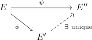
Proof. Omitted (see Silverman, Chapter III, Proposition 4.12). □

Proposition 14.2. Assuming that:

$ϕ : E \to E^{'}$ an isogeny of degree $n$

Then there exists a unique isogeny

\hat{ϕ} : E^{'} \to E

such that

\hat{ϕ} ϕ = [n]

Proof. Case $ϕ$ is separable: We have $| \ker ϕ | = n$ , hence $\ker ϕ \subset E [n]$ . Apply Proposition 14.1 with $ψ = [n]$ .

Case $ϕ$ is inseparable: omitted.

Uniqueness: Suppose $ψ_{1} ϕ = ψ_{2} ϕ = [n]$ . Then $(ψ_{1} - ψ_{2}) ϕ = 0$ , so $\deg (ψ_{1} - ψ_{2}) \deg ϕ = 0$ . Then $\deg (ψ_{1} - ψ_{2}) = 0$ , hence $ψ_{1} = ψ_{2}$ . □

Remark.

(i) Write $E_{1} \sim E_{2}$ to mean “ $E_{1}$ and $E_{2}$ are isogenous”. Then $\sim$ is an equivalence relation.
(ii) $\deg [n] = n^{2}$ gives that $\deg \hat{ϕ} = \deg ϕ$ and $\hat{[n]} = [n]$ .

(iii) Note:

ϕ \hat{ϕ} ϕ = ϕ \circ {[n]}_{E} = {[n]}_{E^{'}} \circ ϕ

Hence $ϕ \hat{ϕ} = {[n]}_{E^{'}}$ .

In particular, $\hat{\hat{ϕ}} = ϕ$ .

(iv) If $E \overset{ψ}{\to} E^{'} \overset{ϕ}{\to} E^{″}$ then $\hat{ϕ ψ} = \hat{ψ} \hat{ϕ}$ .

(v) If

ϕ \in End (E)

then

ϕ^{2} - (Tr ϕ) ϕ + \deg ϕ = 0 .

\underset{= \hat{ϕ}}{\underset{⏟}{([Tr ϕ] - ϕ) ϕ}} = [\deg ϕ] .

Hence $[Tr ϕ] = ϕ + \hat{ϕ}$ .

Lemma 14.3. Assuming that:

$ϕ, ψ \in Hom (E, E^{'})$

Then

\hat{ϕ + ψ} = \hat{ϕ} + \hat{ψ}

Proof.

(i) If $E = E^{'}$ , then this follows from $Tr (ϕ + ψ) = Tr (ϕ) + Tr (ψ)$ .
(ii) In general, let $α : E^{'} \to E$ be any isogeny (e.g. $\hat{ϕ}$ ). Then: $\begin{array}{l} \hat{(α ϕ + α ψ)} & = \hat{α ϕ} + \hat{α ψ} \\ \hat{(ϕ + ψ)} \hat{α} & = (\hat{ϕ} + \hat{ψ}) \hat{α} \end{array}$
Hence the result follows. □

Remark. In Silverman’s book he proves Lemma 14.3first, and uses this to show $\deg : Hom (E, E^{'}) \to ℤ$ is a quadratic form.

Notation.

\begin{array}{l} sum : Div (E) & \to E \\ \underset{formal sum}{\underset{⏟}{\sum n_{p} (P)}} & \mapsto \underset{a d d u s i n g g r o u p l a w}{\underset{⏟}{\sum n_{P} (P)}} \end{array}

Recall

\begin{array}{l} E & \to_{}^{≅} {Pic}^{0} (E) \\ P & \mapsto [(P) - (0)] \end{array}

Therefore $sum D \mapsto [D]$ for all $D \in {Div}^{0} (E)$ .

We deduce:

Lemma 14.4. Assuming that:

$D \in Div (E)$

Then

D \sim 0

if and only if

\deg D = 0

and

sum D = 0_{E}

We will now discuss Weil pairing.

Let $ϕ : E \to E^{'}$ be an isogeny of degree $n$ , with Dual isogeny $\hat{ϕ} : E^{'} \to E$ . Assume $char K ∤ n$ (hence $ϕ$ , $\bar{ϕ}$ separable).

We define the Weil pairing

e_{ϕ} : E [ϕ] \times E^{'} [\hat{ϕ}] \to μ_{n} .

Let $T \in E^{'} [ϕ]$ . Then $n T = 0$ , so there exists $f \in \bar{K} {(E^{'})}^{*}$ such that

div (f) = n (T) - n (0) .

Pick $T_{0} \in E (\bar{K})$ with $ϕ (T_{0}) = T$ . Then

ϕ^{*} (T) - ϕ^{*} (0) = \sum_{P \in E [ϕ]} (P + T_{0}) - \sum_{P \in E [ϕ]} (P)

has sum

n T_{0} = \hat{ϕ} ϕ T_{0} = \hat{ϕ} T = 0 .

So there exists $g \in \bar{K} {(E)}^{*}$ such that

div (g) = ϕ^{*} (T) - ϕ^{*} (0) .

Now

\begin{array}{l} div (ϕ^{*} f) & = ϕ^{*} (div f) \\ = n (ϕ^{*} (T) - ϕ^{*} (0)) \\ = div (g^{n}) \end{array}

Therefore $ϕ^{*} f = c g^{n}$ for some $c \in {\bar{K}}^{*}$ .

Rescaling $f$ , we can say without loss of generality $c = 1$ , i.e. $ϕ^{*} f = g^{n}$ .

For $S \in E [ϕ]$ we get $τ_{S}^{*} (div g) = (div g)$ so $τ_{S}^{*} g = ζ g$ for some $ζ \in {\bar{K}}^{*}$ , i.e. $ζ = \frac{g (X + S)}{g (X)}$ is independent of choice of $X \in E (\bar{K})$ .

Now

ζ^{n} = \frac{g {(X + S)}^{n}}{g {(X)}^{n}} = \frac{f (ϕ (X + S))}{f (ϕ (X))} = 1

since $S \in E [ϕ]$ . Hence $ζ \in μ_{n}$ .

We define

e_{ϕ} (S, T) = \frac{g (X + S)}{g (X)} .

Proposition 14.5. $e_{}$ is bilinear and non-degenerate.

Proof.

(i) Linearity in first argument: $\begin{array}{l} e_{} (S_{1} + S_{2}, T) & = \frac{g (X + S_{1} + S_{2})}{g (X + S_{2})} \frac{g (X + S_{2})}{g (X)} \\ = e_{} (S, T) e_{} (S_{2}, T) \end{array}$
(ii) Linearity in second argument: Let $T_{1}, T_{2} \in E^{'} [\hat{ϕ}]$ . $\begin{array}{l} div (f_{1}) & = n (T_{1}) - n (0) & ϕ^{*} f & = g_{1}^{n} \\ div (f_{2}) & = n (T_{2}) - n (0) & ϕ^{*} f_{2} & = g_{2}^{n} \end{array}$
There exists $h \in \bar{K} (E^{'})$ such that
$div (h) = (T_{1}) + (T_{2}) - (T_{1} + T_{2}) - (0) .$

Then put $f = \frac{f_{1} f_{2}}{h^{n}}$ and $g = \frac{g_{1} g_{2}}{ϕ^{*} h}$ .

Check: $div (f) = n (T_{1} + T_{2}) - n (0)$ . Yes.
$ϕ^{*} f = \frac{ϕ^{*} f_{1} ϕ^{*} f_{2}}{{(ϕ^{*} h)}^{n}} = {(\frac{g_{1} g_{2}}{ϕ^{*} (h)})}^{n} = g^{n} .$

Therefore
$\begin{array}{l} e_{} (S, T_{1} + T_{2}) & = \frac{g (X + S)}{g (X)} \\ = \frac{g_{1} (X + S)}{g_{1} (X)} \frac{g_{2} (X + S)}{g_{2} (X)} \underset{\begin{array}{c} = 1 \\ since S \in E [ϕ] \end{array}}{\underset{⏟}{\frac{h (ϕ (X))}{h (ϕ (X + S))}}} \\ = e_{} (S, T_{1}) e_{} (S, T_{2}) \end{array}$
(iii) $e_{}$ is non-degenerate. Fix $T \in E^{'} [\hat{ϕ}]$ . Suppose $e_{} (S, T) = 1$ for all $S \in E [ϕ]$ . Then $τ_{S}^{*} g = g$ for all $S \in E [ϕ]$ .
Have $\bar{K} (E) ∕ ϕ^{*} \bar{K} (E^{'})$ is a Galois extension with Galois group $E [ϕ]$ ( $S \in E [ϕ]$ acts on $\bar{K} (E)$ via $τ_{S}^{*}$ ).

Therefore $g = ϕ^{*} h$ for some $h \in \bar{K} (E^{'})$ . So $ϕ^{*} f = g^{n} = ϕ^{*} (h^{n})$ . So $f = h^{n}$ , and hence $div (h) = (T) - (0)$ . So $T = 0$ . □

We’ve shown $E^{'} [ϕ] ↪ Hom (E [ϕ], μ_{n})$ . It is an isomorphism since $# E [ϕ] = # E^{'} [\hat{ϕ}] = n$ .

Remark.

(i) If $E, E^{'}, ϕ$ are defined over $K$ then $e_{}$ is Galois equivariant, i.e. $\forall σ \in Gal (\bar{K} ∕ K)$ , $\forall S \in E [ϕ]$ , $\forall T \in E^{'} [ϕ]$ ,
$e_{} (σ S, σ T) = σ (e_{} (S, T)) .$

(ii) Taking

ϕ = [n] : E \to E

(so

\hat{ϕ} = [n]

) gives

e_{n} : E [n] \times E [n] \to μ_{n^{2}} μ_{n} .

Corollary 14.6. Assuming that:

$E [n] \subset E (K)$

Then

μ_{n} \subset K

Proof. Let $T \in E [n]$ have order $n$ . Non degeneracy of $e_{n}$ implies that there exists $S \in E [n]$ such that $e_{n} (S, T)$ is a primitive $n$ -th root of unity, say $ζ_{n}$ .

Then

σ (ζ_{n}) = σ (e_{n} (S, T)) = e_{n} (σ S, σ T) = ζ_{n}

for all $σ \in Gal (\bar{K} ∕ K)$ . So $ζ_{n} \in K$ . □

Example. There does not exist $E ∕ ℚ$ with $E {(ℚ)}_{tors} ≅ {(ℤ ∕ 3 ℤ)}^{2}$ .

Remark. In fact, $e_{n}$ is alternating, i.e. $e_{n} (T, T) = 1$ for all $T \in E [n]$ .

(This implies $e_{n} (S, T) = e_{n} {(T, S)}^{- 1}$ ).

15 Galois Cohomology

Let $G$ be a group and $A$ be a $G$ -module (an abelian group with an action of $G$ via group homomorphisms). $G$ -module means exactly the same thing as $ℤ [G]$ -module.

Definition ( $H^{0}$ ). Define

H^{0} (G, A) = A^{G} = {a \in A | σ (a) = a \forall σ \in G} .

Definition (Cochains). Define

C^{1} (G, A) = {maps G \to A}

(called “cochains”).

Definition (Cocycles). Define

Z^{1} (G, A) = {{(a_{σ})}_{σ \in G} | a_{σ τ} = σ (a_{τ}) + a_{σ} \forall σ, τ \in G}

(called “cocycles”).

Definition (Coboundaries). Define

B^{1} (G, A) = {{(σ b - b)}_{σ \in G} | b \in A}

(called “coboundaries”).

Note. $C^{1} (G, A) \supset Z^{1} (G, A) \supset B^{1} (G, A)$ .

Then we can define:

Definition ( $H^{1}$ ). Define

H^{1} (G, A) = \frac{Z^{1} (G, A)}{B^{1} (G, A)} .

Remark. If $G$ acts trivially on $A$ , then

H^{1} (G, A) = Hom (G, A) .

Theorem 15.1. Assuming that:

we have a short exact sequence of $G$ -modules

$0 \to A \overset{ϕ}{\to} B \overset{ψ}{\to} C \to 0 .$

Then it gives rise to a long exact sequence of abelian groups:

0 \to A^{G} \overset{ϕ}{\to} B^{G} \overset{ψ}{\to} C^{G} \overset{δ}{\to} H^{1} (G, A) \overset{ϕ^{*}}{\to} H^{1} (G, B) \overset{ψ^{*}}{\to} H^{1} (G, C) .

Proof. Omitted. □

Definition ( $d e l t a$ ). Let $c \in C^{G}$ . Then $b \in B$ such that $ψ (b) = c$ . Then

ψ (σ b - b) = σ c - c = 0 \forall σ \in G

so $σ b - b = ϕ (a_{σ})$ for some $a_{σ} \in A$ .

Can check ${(a_{σ})}_{σ \in G} \in Z^{1} (G, A)$ .

Then $δ (c) =$ class of ${(a_{σ})}_{σ \in G}$ in $H^{1} (G, A)$ .

Theorem 15.2. Assuming that:

$A$ is a $G$ -module
$H ⊴ G$ a normal subgroup

Then there is an inflation restriction exact sequence

0 \to H^{1} (G ∕ H, A^{H}) \overset{\inf}{\to} H^{1} (G, A) \overset{res}{\to} H^{1} (H, A)

Proof. Omitted. □

Let $K$ be a perfect field. Then $Gal (\bar{K} ∕ K)$ is a topological group with basis of open subgroups being the $Gal (\bar{K} ∕ L)$ for $[L : K] < \infty$ .

If $G = Gal (\bar{K} ∕ K)$ then we modify the definition of $H^{1} (G, A)$ by insisting:

(1) The stabiliser of each $a \in A$ is an open subgroup of $G$ .
(2) All cochains $G \to A$ are continuous, where $A$ is given the discrete topology.

Then

H^{1} (Gal (\bar{K} ∕ K), A) = \lim_{\begin{array}{c} \to \\ L \\ L ∕ K finite Galois \end{array}} H^{1} (Gal (L ∕ K), A^{Gal (\bar{K} ∕ L)}) .

(direct limit is with respect to inflation maps).

Theorem (Hilbert’s Theorem 90). Assuming that:

$L ∕ K$ a finite Galois extension

Then

H^{1} (Gal (L ∕ K), L^{*}) = 0 .

Proof. Let $G = Gal (L ∕ K)$ . Let ${(a_{σ})}_{σ \in G} \in Z^{1} (G, L^{*})$ . Distinct automorphisms are linearly independent, so there exists $y \in L$ such that

\underset{= x}{\underset{⏟}{\sum_{τ \in G} a_{τ}^{- 1} τ (y)}} \neq 0 .

Then

\begin{array}{l} σ (x) & = \sum_{τ \in G} σ {(a_{τ})}^{- 1} σ τ (y) \\ = a_{σ} \underset{= x}{\underset{⏟}{\sum_{τ \in G} a_{σ τ}^{- 1} σ τ (y)}} \end{array}

Then $a_{σ} = \frac{σ (x)}{x}$ for all $σ \in G$ . ( $a_{σ} τ = σ (a_{τ}) a_{σ}$ $⟹$ $σ {(a_{τ})}^{- 1} = a_{σ} a_{σ τ}^{- 1}$ ).

So ${(a_{σ})}_{σ \in G} \in B^{1} (G, L^{*})$ . Therefore $H^{1} (G, L^{*}) = 0$ . □

Corollary. $H^{1} (Gal (\bar{K} ∕ K), {\bar{K}}^{*}) = 0$ .

Application: Assume $char K ∤ n$ . There is a short exact sequence of $Gal (\bar{K} ∕ K)$ -modules

\begin{array}{l} 0 \to μ_{n} \to {\bar{K}}^{*} & \to {\bar{K}}^{*} \to 0 \\ x & \mapsto x^{n} \end{array}

Long exact sequence:

\begin{array}{l} K^{*} & \to K^{*} \to H^{1} (Gal (\bar{K} ∕ K), μ_{n}) \to \overset{= 0 by Hilbert 90}{\overset{︷}{H^{1} (Gal (\bar{K} ∕ K), {\bar{K}}^{*})}} \\ x & \mapsto x^{n} \end{array}

Therefore $H^{1} (Gal (\bar{K} ∕ K), μ_{n}) ≅ K^{*} ∕ {(K^{*})}^{n}$ .

If $μ_{n} \subset K$ then

{Hom}_{cts} (Gal (\bar{K} ∕ K), μ_{n}) ≅ K^{*} ∕ {(K^{*})}^{n}

Finite subgroups of ${Hom}_{cts} (Gal (\bar{K} ∕ K), μ_{n})$ are of the form $Hom (Gal (L ∕ K), μ_{n})$ for $L ∕ K$ a finite abelian extension of $K$ of exponent dividing $n$ .

This gives another proof of Theorem 11.2.

Notation. $H^{1} (K, -)$ means $H^{1} (Gal (\bar{K} ∕ K), -)$ .

Let $ϕ : E \to E^{'}$ be an isogeny of elliptic curves over $K$ . Short exact sequence of $Gal (\bar{K} ∕ K)$ -modules

0 \to E [ϕ] \to E \overset{ϕ}{\to} E^{'} \to 0

has long exact seqeucne

E (K) \overset{ϕ}{\to} E^{'} (K) \overset{δ}{\to} H^{1} (K, E [ϕ]) \to H^{1} (K, E) \overset{ϕ_{*}}{\to} H^{1} (K, E^{'}) .

We get a short exact sequence

′
0 EϕE(K(K-)) H1 (K,E [ϕ]) H1 (K, E)[ϕ∗] 0

∏ E′(Kv)- ∏ 1 ∏ 1 ∗
δrrδ0esesVvv v ϕE(Kv) vH (Kv,E[ϕ]) vH (Kv, E)[ϕ0]

Now take

K

a number field.

For each place $v$ , fix an embedding $\bar{K} \subset {\bar{K}}_{v}$ . Then $Gal ({\bar{K}}_{v} ∕ K_{v}) \subset Gal (\bar{K} ∕ K)$ .

Definition (Selmer-group). We define the $ϕ$ -Selmer group

\begin{array}{l} S^{(ϕ)} (E ∕ K) & = \ker (H^{1} (K, E [ϕ]) \to \prod_{v} H^{1} (K_{v}, E)) \\ = {α \in H^{1} (K, E [ϕ]) | {res}_{v} (α) \in Im (δ_{v}) \forall v} \end{array}

(the map $H^{1} (K, E [ϕ]) \to \prod_{v} H^{1} (K_{v}, E)$ is as in the commutative diagram above).

Definition (Tate-Shafarevich group). The Tate-Shafarevich group is

T S (E ∕ K) = \ker (H^{1} (K, E) \to \prod_{v} H^{1} (K_{v}, E)) .

We get a short exact sequence

0 \to \frac{E^{'} (K)}{ϕ E (K)} \to S^{(ϕ)} (E ∕ K) \to T S (E ∕ K) [ϕ_{K}] \to 0 .

Taking $ϕ = [n]$ gives

0 \to \frac{E (K)}{n E (K)} \to S^{(n)} (E ∕ K) \to T S (E ∕ K) [n] \to 0 .

Reorganising the proof of Mordell-Weil gives

Theorem 15.3. $S^{(n)} (E ∕ K)$ is finite.

Proof. For $L ∕ K$ a finite Galois extension,

finite
◜-1------◞◟--------◝
0 H (Gal(L∕K ),E(L)[n ]) H1 (K,E [n]) H1(L,E [n])

inr⊃⊃fes S (n)(E ∕K ) S(n)(E∕L )

Therefore by extending our field, we may assume

E [n] \subset E (K)

and hence by the Weil pairing

μ_{n} \subset K

Therefore $E [n] ≅ μ_{n} \times μ_{n}$ as a $Gal (\bar{K} ∕ K)$ -module. Then

\begin{array}{l} H^{1} (K, E [n]) & ≅ H^{1} (K, μ_{n}) \times H^{1} (K, μ_{n}) \\ ≅ K^{*} ∕ {(K^{*})}^{n} \times K^{*} ∕ {(K^{*})}^{n} \end{array}

Let

S = {primes of bad reduction for E} \cup {v | n \infty}

(a finite set of places).

Define the subgroup of $H^{1} (K, A)$ unramified outside of $S$ as

H^{1} (K, A; S) = \ker (H^{1} (K, A) \to \prod_{v \notin S} H^{1} (K_{v}^{nr}, A)) .

There is a commutative diagram with exact rows:

E (Kv ) E(Kv ) H1(Kv,E [n])

×δr×0nvesn E (Knrv ) E(Kvnr ) H1(Knrv ,E [n])

The bottom map

\times n

is surjective

\forall v \notin S

(see Theorem 9.8).

Therefore

\begin{array}{l} S^{(n)} (E ∕ K) & \subset H^{1} (K, E [n]; S) \\ ≅ H^{1} (K, μ_{n}; S) \times H^{1} (K, μ_{n}; S) \end{array}

But

\begin{array}{l} H^{1} (K, μ_{n}; S) & = \ker (\frac{K^{*}}{{(K^{*})}^{n}} \to \prod_{v \notin S} \frac{{(K_{v}^{nr})}^{*}}{{(K_{v}^{nr})}^{* n}}) \\ \subset K (S, n) \end{array}

which is finite by Lemma 11.4. □

Remark. $S^{(n)} (E ∕ K)$ is finite and effectively computable.

It is conjectured that $| T S (E ∕ K) | < \infty$ . This would imply that $rank E (K)$ is effectively computable.

16 Descent by Cyclic Isogeny

Let $E, E^{'}$ be elliptic curves over a number field $K$ , and $ϕ : E \to E^{'}$ an isogeny of degree $n$ .

Suppose $E^{'} [\hat{ϕ}] ≅ ℤ ∕ n ℤ$ generated by $T \in E^{'} (K)$ . Then $E [ϕ] ≅ μ_{n}$ as a $Gal (\bar{K} ∕ K)$ -module

S \mapsto e_{} (S, T) .

Have a short exact sequence of $Gal (\bar{K} ∕ K)$ -modules

0 \to μ_{n} \to E \overset{ϕ}{\to} E^{'} \to 0 .

Get long exact sequence

E (K ) E ′(K ) H1(K, μn) H1 (K,E )

ϕδα∼= K∗∕(K ∗)n

(the

≅

is by Hilbert 90).

Theorem 16.1. Assuming that:

$f \in K (E^{'})$ and $g \in K (E)$
$div (f) = n (T) - n (0)$
$ϕ^{*} f = g^{n}$

Then

α (P) = f (P) (m o d {(K^{*})}^{n})

for all

P \in E; (K) ∖ {0, T}

Proof. Let $Q \in ϕ^{- 1} P$ . Then $δ (P) \in H^{1} (K, μ_{n})$ is represented by $σ \mapsto σ Q - Q \in E [ϕ] ≅ μ_{n}$ .

\begin{array}{l} e_{} (σ Q - Q, T) & = \frac{g (σ Q - Q + X)}{g (X)} & \begin{array}{c} for any X \in E \\ avoiding zeroes and poles of g \end{array} \\ = \frac{g (σ Q)}{g (Q)} & pick X = Q \\ = \frac{σ (g (Q))}{g (Q)} \\ = \frac{σ \sqrt[n]{f (P)}}{\sqrt[n]{f} (P)} \end{array}

( $ϕ^{*} f = g^{n}$ , $f (P) = g {(Q)}^{n}$ ).

But

\begin{array}{l} H^{1} (K, μ_{n}) & ≅ K^{*} ∕ {(K^{*})}^{n} \\ (σ \mapsto \frac{\sqrt[n]{x}}{\sqrt[n]{x}}) & \leftarrow ↤ x \end{array}

Hence $α (P) = f (P) (m o d {(K^{*})}^{n})$ . □

16.1 Descent by 2-isogeny

\begin{array}{l} E : & y^{2} = x (x^{2} + a x + b) \\ E^{'} : & y^{2} = x (x^{2} + a^{'} x + b^{'}) \end{array}

b (a^{2} - 4 b) \neq 0

a^{'} = - 2 a

b^{'} = a^{2} - 4 b

\begin{array}{l} ϕ : E & \to E^{'} \\ (x, y) & \mapsto ({(\frac{y}{x})}^{2}, \frac{y (x^{2} - b)}{x^{2}}) \\ \hat{ϕ} : E^{'} & \to E \\ (x, y) & \mapsto (\frac{1}{4} {(\frac{y}{x})}^{2}, \frac{y (x^{2} - b^{'})}{8 x^{2}}) \end{array}

$E [ϕ] = {0, T}$ , $T = (0, 0) \in E (K)$ .

$E^{'} [\hat{ϕ}] = {0, T^{'}}$ , $T^{'} = (0, 0) \in E^{'} (K)$ .

Proposition 16.2. There is a group homomorphism

\begin{array}{l} E^{'} (K) & \to K^{*} ∕ {(K^{*})}^{2} \\ (x, y) & \mapsto {\begin{matrix} x mod {(K^{*})}^{2} & if x \neq 0 \\ b^{'} mod {(K^{*})}^{2} & if x = 0 \end{matrix} \end{array}

with kernel $ϕ E (K)$ .

Proof. Either: Apply Theorem 16.1 with $f = x \in K (E^{'})$ , $g = \frac{y}{x} \in K (E)$ .

Or: direct calculation – see Example Sheet 4. □

\begin{array}{l} α_{E} : \frac{E (K)}{\hat{ϕ} E^{'} (K)} & ↪ K^{*} ∕ {(K^{*})}^{2} \\ α_{E^{'}} : \frac{E^{'} (K)}{ϕ E (K)} & ↪ K^{*} ∕ {(K^{*})}^{2} \end{array}

Lemma 16.3. $2^{rank E (K)} = \frac{| Im α_{E} | \cdot | Im α_{E^{'}} |}{4}$ .

Proof. If $A \overset{f}{\to} B \overset{g}{\to} C$ are homomorphisms of abelian groups, then there is an exact sequence

0 ker(f) ker(gf ) ker(g)

fg coker(f) coker(gf) coker(g) 0

Since

\hat{ϕ} ϕ = {[2]}_{E}

, we get an exact sequence

0 \to \underset{≅ ℤ ∕ 2 ℤ}{\underset{⏟}{E (K) [ϕ]}} \to E (K) [2] \overset{ϕ}{\to} \underset{≅ ℤ ∕ 2 ℤ}{\underset{⏟}{E^{'} (K) [ϕ^{'}]}} \to \underset{≅ Im (α_{E^{'}})}{\underset{⏟}{\frac{E^{'} (K)}{ϕ E (K)}}} \overset{\hat{ϕ}}{\to} \frac{E (K)}{2 E (K)} \to \underset{≅ Im (α_{E})}{\underset{⏟}{\frac{E (K)}{\hat{ϕ} E^{'} (K)}}} \to 0 .

Therefore

\frac{| E (L) ∕ 2 E (K) |}{| E (K) [2] |} = \frac{| Im α_{E} | \cdot | Im α_{E^{'}} |}{4} . (1)

Mordell-Weil: $E (K) ≅ Δ \times ℤ^{r}$ , where $Δ$ is a finite group and $r = rank E (K)$ .

$\frac{E (K)}{2 E (K)} ≅ \frac{Δ}{2 Δ} \times {(\frac{ℤ}{2 ℤ})}^{r}$ .

$E (K) [2] ≅ Δ [2]$ .

Since $Δ$ is finite, we have that $\frac{Δ}{2 Δ}$ and $Δ [2]$ have the same order, and therefore

\frac{| E (K) ∕ 2 E (K) |}{| E (K) [2] |} = 2^{r} . (2)

So we are done, by using (1) and (2). □

Lemma 16.4. Assuming that:

$K$ is a number field
$a, b \in O_{K}$

Then

Im (α_{E}) \subset K (S, 2)

, where

S = {𝔭 | b}

Proof. We must show that $x, y \in K$ , $y^{2} = x (x^{2} + a x + b)$ and $v_{𝔭} (b) = 0$ then $v_{𝔭} (x) \equiv 0 (m o d 2)$ .

Case $v_{𝔭} (x) < 0$ : Lemma 9.1 gives that for some $r \geq 1$ , $v_{𝔭} (x) = - 2 r$ and $v_{𝔭} (y) = - 3 r$ , so done.

Case $v_{𝔭} (x) > 0$ : Then $v_{𝔭} (x^{2} + a x + b) = 0$ . So $v_{𝔭} (x) = v_{𝔭} (y^{2}) = 2 v_{𝔭} (y)$ . □

Lemma 16.5. Assuming that:

$b_{1} b_{2} = b$

Then

b_{1} (K^{*}) \in Im (α_{E})

if and only if

w^{2} = b_{1} u^{4} + a u^{2} v^{2} + b_{2} v^{4} (∗)

is soluble for $u, v, w \in K$ not all zero.

Proof. If $b_{1} \in {(K^{*})}^{2}$ or $b_{2} \in {(K^{*})}^{2}$ then both conditions are satisfied. So we may assume $b_{1}, b_{2} \notin {(K^{*})}^{2}$ .

Now note $b_{1} {(K^{*})}^{2} \in Im (α_{E})$ if and only if there exists $(x, y) \in E (K)$ such that $x = b_{1} t^{2}$ for some $t \in K^{*}$ . This implies

y^{2} = (b_{1} t^{2}) (b_{1}^{2} t^{2} + a b_{1} t^{2} + b)

hence

{(\frac{y}{b_{1} t})}^{2} = b_{1} t^{4} + a t^{2} + \underset{= b_{2}}{\underset{⏟}{\frac{b}{b_{1}}}} .

So ( $*$ ) has solution $(u, v, w) = (t, 1, \frac{y}{b_{1} t})$ .

Conversely, if $(u, v, w)$ is a solution to ( $*$ ) then $u v \neq 0$ and $(b_{1} {(\frac{u}{v})}^{2}, b_{1} \frac{u w}{v^{3}}) \in E (K)$ . □

Now take $K = ℚ$ .

Example. $E$ : $y^{2} = x^{3} - x$ ( $a = 0$ , $b = - 1$ ).

$Im (α_{E}) = ⟨ - 1 ⟩ \subset ℚ^{*} ∕ {(ℚ^{*})}^{2}$ .

$E^{'}$ : $y^{2} = x^{3} + 4 x$ .

$Im (α_{E^{'}}) \subset ⟨ - 1, 2 ⟩ \subset ℚ^{*} ∕ {(ℚ^{*})}^{2}$ .

\begin{array}{l} b_{1} & = - 1 & w^{2} & = - u^{4} - 4 v^{4} \\ b_{1} & = 2 & w^{2} & = 2 u^{4} + 2 v^{4} \\ b_{1} & = - 2 & w^{2} & = - 2 u^{4} - 2 v^{4} \end{array}

The first and last lines are insoluble over

ℝ

(squares are non-negative). The middle line does have a solution:

(u, v, w) = (1, 1, 2)

Therefore $Im (α_{E^{'}}) = ⟨ 2 ⟩ \subset ℚ^{*} ∕ {(ℚ^{*})}^{2}$ .

Hence $2^{rank E (ℚ)} = \frac{2 \cdot 2}{4} = 1$ , so $rank E (ℚ) = 0$ .

So $1$ is not a congruent number.

Example. $E$ : $y^{2} = x^{3} + p x$ , $p$ a prime which is 5 modulo 8.

\begin{array}{l} b_{1} & = - 1 & w^{2} & = - u^{4} - p v^{4} \end{array}

This is insoluble over $ℝ$ , hence $Im (α_{E}) = ⟨ p ⟩ \subset ℚ^{*} ∕ {(ℚ^{*})}^{2}$ .

$E^{'}$ : $y^{2} = x^{3} - 4 p x$ .

$Im (α_{E^{'}}) \subset ⟨ - 1, 2, p ⟩ \subset ℚ^{*} ∕ {(ℚ^{*})}^{2}$ .

Note: $α_{E^{'}} (T^{'}) = (- 4 p) {(ℚ^{*})}^{2} = (- p) {(ℚ^{*})}^{2}$ .

\begin{array}{l} b_{1} & = 2 & w^{2} & = 2 u^{4} - 2 p v^{4} \\ b_{1} & = 2 & w^{2} & = - 2 u^{4} + 2 p v^{4} \\ b_{1} & = p & w^{2} & = p u^{4} - 4 v^{4} \end{array}

Suppose the first line is soluble. Then without loss of generality $u, v, w \in ℤ$ with $\gcd (u, v) = 1$ . If $p | u$ , then $p | w$ and then $p | v$ , contradiction. Therefore $w^{2} \equiv 2 u^{4} ⁄ \equiv 0 (m o d p)$ . So $(\frac{2}{p}) = + 1$ , which contradicts $p \equiv 5 (m o d 8)$ .

Likewise the second line has no solution since $(\frac{- 2}{p}) = - 1$ .

TODO

Example (Lindemann). $E$ : $y^{2} = x^{3} + 17 x$ .

Im (α_{E}) = ⟨ 17 ⟩ \subset ℚ^{*} ∕ {(ℚ^{*})}^{2} .

$E^{'}$ : $y^{2} = x^{3} - 68 x$ .

Im (α_{E^{'}}) \subset ⟨ - 1, 2, 17 ⟩ \subset ℚ^{*} ∕ {(ℚ^{*})}^{2} .

$b_{1} = 2$ , $w^{2} = 2 u^{4} - 34 v^{4}$ .

Replacing $w$ by $2 w$ and dividing by $2$ gives

C : 2 w^{2} = u^{4} - 17 v^{4} .

Notation. $C (K) = {(u, v, w) \in K^{3} ∖ {0} satisfying equation above} ∕ \sim$ , where $(u, v, w) \sim (λ u, λ v, λ^{2} w)$ for all $λ \in K^{*}$ .

$C (ℚ_{2}) \neq \emptyset$ since $17 \in {(ℤ_{2}^{*})}^{4}$ .

$C (ℚ_{17}) \neq \emptyset$ since $2 \in {(ℤ_{17}^{*})}^{2}$ .

$C (ℝ) \neq \emptyset$ since $\sqrt{2} \in ℝ$ .

Therefore $C (ℚ_{v}) \neq \emptyset$ for all places $v$ of $ℚ$ .

Suppose $(u, v, w) \in C (ℚ)$ . Without loss of generality say $u, v, w \in ℤ$ , $\gcd (u,, v) = 1$ and $w > 0$ .

If $17 | w$ then $17 | u$ and then $17 | v$ , contradiction

So if $p | w$ then $p \neq 17$ and $(\frac{17}{p}) = + 1$ . Therefore $(\frac{p}{17}) = (\frac{17}{p}) = 1$ (using quadratic reciprocity). (If $p$ is odd, also $(\frac{2}{17}) = + 1$ ).

Therefore $(\frac{w}{17}) = + 1$ . But $2 w^{2} \equiv u^{4} (m o d 17)$ , so $2 \in {(𝔽_{17}^{*})}^{4} = {\pm 1, \pm 4}$ , contradiction.

So $C (ℚ) = \emptyset$ , i.e. $C$ is a counterexample to the Hasse Principle. It represents a non-trivial element of $T S (E ∕ ℚ)$ .

16.2 Birch Swinnerton Dyer Conjecture

Let $E ∕ ℚ$ be an elliptic curve.

Definition ( $L (E, s)$ ). Define

L (E, s) = \prod_{p} L_{p} (E, s)

where

L_{p} (E, s) = {\begin{matrix} {(1 - a_{p} p^{- s} + p^{1 - 2 s})}^{- 1} & if good reduction \\ {(1 - p^{- s})}^{- 1} & if split multiplicative reduction \\ {(1 + p^{- s})}^{- 1} & if nonsplit multiplicative reduction \\ 1 & if additive reduction \end{matrix}

where $# Ẽ (𝔽_{p}) = 1 + p - a_{p}$ .

Hasse’s Theorem implies $| a_{p} | \leq 2 \sqrt{p}$ , which shows that $L (E, s)$ converges for $Re (s) > \frac{3}{2}$ .

Theorem (Wiles, Breuil, Conrad, Diamon, Taylor). $L (E, s)$ is the $L$ -function of a weight $2$ modular form, and hence has an analytic continuation to all of $ℂ$ (and a function equation relating $L (E, s) = L (E, 2 - s)$ ).

Conjecture (Weak Birch Swinnerton-Dyer Conjecture). ${ord}_{s = 1} L (E, s) = rank E (ℚ)$ .

( $= r$ say).

Conjecture (Strong Birch Swinnerton-Dyer Conjecture). ${ord}_{s = 1} L (E, s) = rank E (ℚ)$ , which we shall call $r$ , and

\lim_{s \to 1} \frac{1}{{(s - 1)}^{r}} L (E, s) = \frac{Ω_{E} Reg E (ℚ) | T S (E ∕ ℚ) | \prod_{p} c_{p} (E)}{| E {(ℚ)}_{tors} |^{2}},

where

$c_{p}$ is given by:
$\begin{array}{l} c_{p} (E) & = Tamagawa number of E ∕ ℚ_{p} \\ = [E (ℚ_{p}) : E_{0} (ℚ_{p})] \end{array}$

If $E (ℚ) ∕ E {(ℚ)}_{tors} = ⟨ P_{1}, P_{2}, \dots, P_{r} ⟩$ , then $Reg E (ℚ) = \det {([P_{i}, P_{j}])}_{i, j = 1, \dots, r}$ , where

[P, Q] = ĥ (P + Q) - ĥ (P) - ĥ (Q) .

$Ω_{E}$ is given by:
$Ω_{E} = \int_{E (ℝ)} | \frac{d x}{2 y + a_{1} x + a_{3}} |,$

where $a_{1}, \dots, a_{6} \in ℤ$ are coefficients of a globally minimal Weierstrass equation for $E ∕ ℚ$ .