Analytic Number Theory - Cambridge III notes

Analytic Number Theory
Daniel Naylor

1Estimating Primes
1.1Asymptotic Notation
1.2Partial Summation
1.3Arithmetic Functions and Dirichlet convolution
1.4Dirichlet Series
2Elementary Estimates for Primes
2.1Merten’s Theorems
2.2Sieve Methods
2.3Selberg Sieve
3The Riemann Zeta Function
3.1Partial fraction approximation of

ζ

3.2Zero-free region
Index

What is analytic number theory?

Study of number-theoretic problems using analysis (real, complex, Fourier, …)
Also tools from combinatorics, probability, …

What kind of problems are studied?

A variety of problems about integers, especially primes.

Are there infinitely many primes? (Euclid, 300BC)
Are there infinitely many primes starting with 7 in base 10? (follows from prime number theorem)
Are there infinitely many primes ending with 7 in base 10? (follows from Dirichlet’s theorem)
Are there infinitely many primes with 49% of the digits being 7 in base 10? would follow from the Riemann hypothesis
Are there infinitely many pairs of primes differing by 2? (twin prime conjecture)

Key feature: To show that a set (of primes) is infinite, want to estimate the number of elements $\leq x$ .

Definition. Define

π (x) = | {primes \leq x} | = \sum_{p \leq x} 1 .

Euclid showed: $\lim_{x \to \infty} π (x) = \infty$ .

Theorem (Prime number theorem).

\lim_{x \to \infty} \frac{π (x) \log x}{x} = 1 .

$π (x) \sim \frac{x}{\log x}$ . (Conjectured: Legendre, Gauss. Proved: Hadamard, de la Vallée Poussin)

1 Estimating Primes

Theorem (Euler). $\sum_{p} \frac{1}{p} = \infty$ .

Proof. Consider $p_{N} = \prod_{p}^{N} (1 + \frac{1}{p} + \frac{1}{p^{2}} + \dots + \frac{1}{p^{N}})$ , for $N \in ℕ = {1, 2, 3, \dots}$ . We have:

\begin{array}{l} p_{N} & \geq \sum_{n = 1}^{N} \frac{1}{n} \\ \geq \sum_{n = 1}^{N - 1} \int_{n}^{n + 1} \frac{d t}{t} \\ = \int_{1}^{N - 1} \frac{d t}{t} \\ = \log (N - 1) \end{array}

On the other hand, using $1 + x \leq e^{x}$ , so

\begin{array}{l} p_{N} & \leq \prod_{p \leq N} \exp (\frac{1}{p} + \frac{1}{p^{2}} + \dots + \frac{1}{p^{N}}) \\ = \exp (\sum_{p \leq N} (\frac{1}{p} + \frac{1}{p^{2}} + \dots + \frac{1}{p^{N}})) \\ \leq \exp (\sum_{p \leq N} (\frac{1}{p} + \frac{1}{p^{2} - p})) \\ \leq \exp (C + \sum_{p \leq N} \frac{1}{p}) \end{array}

Comparing these two bounds gives

\sum_{p \leq N} \frac{1}{p} \geq \log \log (N - 1) - C .

Then letting $N \to \infty$ gives the desired result. □

Theorem (Chebyshev’s Theorem).

π (x) \leq \frac{c x}{\log x}

(for $x \geq 2$ , where $c$ is an absolute constant).

Proof. Consider

\begin{array}{l} S_{N} & = (\binom{2 N}{N}) \\ = \frac{(2 N)!}{{(N!)}^{2}} \end{array}

for $N \in ℕ$ . We have

S_{N} \leq \sum_{j = 0}^{2 N} (\binom{2 N}{j}) = {(1 + 1)}^{2 N} = 4^{N} .

On the other hand,

S_{N} = \prod_{p \leq 2 N} p^{α^{p} (N)}

where $α_{p} (N)$ is the largest $j$ such that $p^{j} | (\binom{2 N}{N})$ . We have $α_{p} (N) = 1$ for $p \in (N, 2 N]$ . So

(\log 4) N \geq \sum_{N < p \leq 2 N} \log p .

Take $N = ⌈ \frac{x}{2} ⌉$ , for $x \geq 2$ . Hence

\sum_{x < p \leq 2 x} \log p \leq (\log 4) ⌈ \frac{x}{2} ⌉ + \log x \leq (\log 4) \frac{x}{2} + \log 4 + \log x .

Then

\begin{array}{l} \sum_{p \leq x} & \leq \sum_{0 \leq j \leq \frac{\log x}{\log 2}} ((\log 4) \frac{x}{2^{j + 2}} + \log x) & (telescoping summation, take \frac{x}{2}, \frac{x}{2^{2}}, \frac{x}{2^{3}}, \dots) \\ \leq (\log 4) x + {(\log x)}^{2} + 1 \end{array}

So for $x \geq 2$ and a suitable large enough constant $c^{'}$ , we have

\sum_{p \leq x} \leq (\log 4) x + c^{'} {(\log x)}^{2} .

Hence

\begin{array}{l} \sum_{\frac{x}{{(\log x)}^{2}} < p \leq x} \log p & \leq (\log 4) x + c^{'} {(\log x)}^{2} \\ ⟹ \log \frac{x}{{(\log x)}^{2}} (π (x) - π (\frac{x}{{(\log x)}^{2}})) & \leq (\log 4) x + c^{'} {(\log x)}^{2} \\ ⟹ π (x) & \leq \frac{x}{{(\log x)}^{2}} + (\log 4) \frac{x}{\log \frac{x}{{(\log x)}^{2}}} + c^{'} \frac{{(\log x)}^{2}}{\log \frac{x}{{(\log x)}^{2}}} \\ \leq (\log 4 + 𝜀) \frac{x}{\log x} \end{array}

for any $𝜀$ , as long as $x \geq x (𝜀)$ .

Take $𝜀 = 1$ . Choose $c > 0$ large enough. □

1.1 Asymptotic Notation

Definition 1.1 (Big $O$ and little $o$ notation). Let $f, g, h : S \to ℂ$ , $S \subseteq ℂ$ .

Write $f (x) = O (g (x))$ if there is $c > 0$ such that $| f (x) | \leq c | g (x) |$ for all $x \in S$ .

Write $f (x) = o (g (x))$ if for any $𝜀 > 0$ there is $x_{𝜀} > 0$ such that $| f (x) | \leq 𝜀 | g (x) |$ for $x \in S$ , $| x | \geq x_{𝜀}$ .

Write $f (x) = g (x) + O (h (x))$ if $f (x) - g (x) = O (h (x))$ and write $f (x) = g (x) + o (h (x))$ if $f (x) - g (x) = o (h (x))$ .

Definition 1.2 (Vinogradov notation). Let $f, g, h : S \to ℂ$ , $S \subseteq ℂ$ .

Write $f (x) ≪ g (x)$ or $g (x) ≫ f (x)$ if $f (x) = O (g (x))$ .

Example.

${(\log x)}^{1} 00 ≪ \exp (\sqrt{\log x}) ≪ x^{\frac{1}{100}}$ ( $x \leq 1$ ), since $\lim_{x \to \infty} \frac{{(\log x)}^{100}}{\exp (\sqrt{\log x})} = 0$ , $\lim_{x \to \infty} \frac{\exp (\sqrt{\log x})}{x^{\frac{1}{100}}} = 0$ .
$100 x + 100 ≪ x ≪ \frac{x}{100}$ (for $x \geq 1$ ).
$e^{x} = 1 + x + O (x^{2})$ for $x \in [- 10, 10]$ , since $e^{x} = 1 + x + \sum_{n = 2}^{\infty} \frac{x^{n}}{n!}$ .
$⌊ x ⌋ = x + O (1)$ for $x \in ℝ$ (since $⌊ x ⌋ \in (x - 1, x]$ ).
$\frac{x + 1}{x} = 1 + o (1)$ (for $x \geq 1$ ).

Lemma. Let $f, g, h, u : S \to ℂ$ .

(i) If $f (x) = O (g (x))$ and $g (x) = O (h (x))$ , then $f (x) = O (h (x))$ (transitivity).
(ii) If $f (x) = O (h (x))$ and $g (x) = O (u (x))$ , then $f (x) + g (x) = O (| h (x) | + | u (x) |)$ .
(iii) If $f (x) = O (h (x))$ and $g (x) = O (u (x))$ , then $f (x) g (x) = O (h (x) u (x))$ .

Proof. Follows from the definition in a straightforward way. Example:

(iii) $| f (x) | \leq c_{1} | h (x) |$ , $| g (x) | \leq c_{2} | u (x) |$ . Then $| f (x) g (x) | \leq c_{1} c_{2} | h (x) u (x) |$ , so $f (x) g (x) = O (h (x) u (x))$ . □

1.2 Partial Summation

Lemma 1.3 (Partial Summation). Assuming that:

${(a_{n})}_{n \in ℕ}$ are complex numbers
$x \geq y \geq 0$
$f : [y, x] \to ℂ$ is continuously differentiable

Then

\sum_{y < n \leq x} a_{n} f (n) = A (x) f (x) - A (y) f (y) - \int_{y}^{x} A (t) f^{'} (t) d t,

where for $t \geq 1$ , we define

A (t) = \sum_{n \leq t} a_{n} = \sum_{n = 1}^{⌊ t ⌋} a_{n} .

Proof. It suffices to prove the $y = 0$ case, since then

\sum_{y < n \leq x} a_{n} f (n) = \sum_{0 < n \leq x} a_{n} f (n) - \sum_{0 < n \leq y} a_{n} f (n) .

Suppose $y = 0$ . By the fundamental theorem of calculus,

f (n) = f (x) - \int_{n}^{x} f^{'} (t) d t = \int_{0}^{x} f^{'} (t) 𝟙_{[n, x]} (t) d t .

Summing over $n \leq x$ , we get

\begin{array}{l} \sum_{n \leq x} a_{n} f (n) & = A (x) f (x) - \int_{0}^{x} f^{'} (t) (\sum_{n \leq x} 𝟙_{[n, x]} (t) a_{n}) d t \\ = A (x) f (x) - \int_{0}^{x} f^{'} (t) A (t) d t □ \end{array}

Lemma. If $x \geq 1$ , then

\sum_{n \leq x} \frac{1}{n} = \log x + γ + O (\frac{1}{x}),

where $γ \in ℝ$ is Euler’s constant, which is given by $γ = \lim_{N \to \infty} \sum_{k = 1}^{N} \frac{1}{k} - \log N$ .

Proof. Apply Partial Summation with $a_{n} = 1$ , $f (t) = \frac{1}{t}$ , $y = \frac{1}{2}$ . Clearly $A (t) = ⌊ t ⌋$ . Then,

\begin{array}{l} \sum_{n \leq x} \frac{1}{n} & = \frac{⌊ x ⌋}{x} + \int_{1}^{x} \frac{⌊ t ⌋}{t^{2}} d t \\ = \frac{x + O (1)}{x} + \int_{1}^{x} \frac{t - {t}}{t^{2}} d t \\ = 1 + O (\frac{1}{x}) + \log x - \int_{1}^{x} \frac{{t}}{t^{2}} d t \\ = 1 + \log x - \int_{1}^{\infty} \frac{{t}}{t^{2}} d t + O (\frac{1}{x}) \end{array}

The last equality is true since $\int_{x}^{\infty} \frac{{t}}{t^{2}} d t \leq \int_{x}^{\infty} \frac{1}{t^{2}} d t = \frac{1}{x}$ .

Let $γ = 1 - \int_{1}^{\infty} \frac{{t}}{t^{2}} d t$ . Then we have the asymptotic equation as desired.

Taking $x \to \infty$ in the formula, we see that $γ$ is equal to the formula for Euler’s constant, as desired. □

Lemma. For $x \geq 1$ ,

\sum_{p \leq x} \frac{1}{p} = \int_{1}^{x} \frac{π (t)}{t^{2}} d t + O (1) .

Proof. Apply Lemma 1.3 with $a_{n} = 𝟙_{ℙ} (n)$ (where $ℙ$ is the set of primes), $f (t) = \frac{1}{t}$ , and $y = 1$ .

We get $A (t) = π (t)$ , and then

\begin{array}{l} \sum_{p \leq x} \frac{1}{p} & = \frac{π (x)}{x} + \int_{1}^{x} \frac{π (t)}{t^{2}} d t \\ = \int_{1}^{x} \frac{π (t)}{t^{2}} d t + O (1) □ \end{array}

1.3 Arithmetic Functions and Dirichlet convolution

Definition (Arithmetic function). An arithmetic function is a function $f : ℕ \to ℂ$ .

Definition (Multiplicative). An arithmetic function $f$ is multiplicative if $f (1) = 1$ and $f (m n) = f (m) f (n)$ whenever $m, n \in ℕ$ are coprime.

Moreover, $f$ is completely multiplicative if $f (m n) = f (m) f (n)$ for all $m, n$ .

Example.

$f (n) = n^{s}$ for $s \in ℂ$ is completely multiplicative.
Möbius function
$μ (n) = {\begin{matrix} 1 & n = 1 \\ {(- 1)}^{k} & if n is a product of k distinct primes \\ 0 & n is divisible by a square of a prime \end{matrix}$

This is multiplicative:
- If $μ (m n) = 0$ and $m$ , $n$ are coprime, then we must have had at least one of $μ (m) = 0$ or $μ (n) = 0$ .
- If $μ (m n) = 1$ , then say $m$ is a product of $k$ distinct primes and $n$ is a product of $l$ distinct primes. Then $μ (m n) = {(- 1)}^{k + l} = {(- 1)}^{k} {(- 1)}^{l} = μ (m) μ (n)$ .
- $τ (n) = \sum_{n = a b} 1$ (divisor function) and $τ_{k} (n) = \sum_{n = n_{1} n_{2} \dots n_{k}} 1$ (generalised divisor function). $τ$ and $τ_{k}$ are multiplicative.

On the space of arithmetic functions, we have operations:

\begin{array}{l} (f + g) (n) & = f (n) + g (n) \\ (f g) (n) & = f (n) g (n) \\ (f * g) (n) & = Dirichlet convolution \end{array}

Definition (Dirichlet convolution). For $f, g : ℕ \to ℂ$ , we define

(f * g) (n) = \sum_{d | n} f (d) g (\frac{n}{d}),

where $\sum_{d | n}$ means sum over the divisors of $n$ .

Lemma 1.4. The space of arithmetic functions with operations $+$ , $*$ is a commutative ring.

Proof. Since arithmetic functions with $+$ form an abelian group, it suffices to show:

(i) $(f * g) * h = f * (g * h)$
(ii) $f * g = g * f$
(iii) $f * I = f$
(iv) $f * (g + h) = f * g + f * h$

Proofs:

(i) Follows from $(f * g) (n) = \sum_{n = a b} f (a) g (b)$ .
(ii) Follows from $(f * g) (n) = \sum_{n = a b} f (a) g (b)$ .
(iii) Take
$I (n) = {\begin{matrix} 1 & n = 1 \\ 0 & n \neq 0 \end{matrix} .$

Then one can check that $f * I = f$ .
(iv) From definition. □

Lemma. The set of arithmetic functions $f$ with $f (1) \neq 0$ form an abelian group with operation $*$ .

Proof. Need $g$ such that $f * g = I$ .

(f * g) (1) = f (1) g (1) = 1 ⟹ g (1) = \frac{1}{f (1)} .

Assume $g (m)$ defined for $m < n$ . We will defined $g (n)$ .

\begin{array}{l} (f * g) (n) & = g (n) f (1) + \sum_{\begin{array}{c} d | n \\ d \neq 1 \end{array}} f (d) g (\frac{n}{d}) \\ ⟹ g (n) & = - \frac{1}{f (1)} \sum_{\begin{array}{c} d | n \\ d \neq 1 \end{array}} f (d) g \underset{< n}{\underset{⏟}{(\frac{n}{d})}} □ \end{array}

Lemma. Multiplicative arithmetic functions form an abelian group with $*$ . Moreover, for completely multiplicative $f$ , the Dirichlet inverse is $μ f$ .

Proof. For the first part, suffices to show closedness. Let $f, g : ℕ \to ℂ$ be multiplicative, and $m, n$ coprime.

If $m n = a b$ , we can write $a = a_{1} a_{2}$ , $b = b_{1} b_{2}$ where $a_{1} = (a, m)$ , $a_{2} = (a, n)$ , $b_{1} = (b, m)$ and $b_{2} = (b, n)$ . Therefore we have:

\begin{array}{l} (f * g) (m n) & = \sum_{m n = a b} f (a) g (b) \\ = \sum_{\begin{array}{c} m = a_{1} b_{1} \\ n = a_{2} b_{2} \end{array}} f (a_{1} a_{2}) g (b_{1} b_{2}) & (above observation) \\ = \sum_{\begin{array}{c} m = a_{1} b_{1} \\ n = a_{2} b_{2} \end{array}} f (a_{1}) f (a_{2}) g (b_{1}) g (b_{2}) & (by multiplicativity) \\ = (f * g) (m) (f * g) (n) \end{array}

(also need to check that inverses are multiplicative).

Now, remains to show that for completely multiplicative $f$ , $f * μ f = I$ .

Note that $f * μ f$ is multiplicative by the first part. So enough to show $(f * μ f) (p^{k}) = I (p^{k})$ for prime powers $p^{k}$ . Calculate:

\begin{array}{l} f * μ f (p) & = f (p) + μ f (p) \\ = f (p) - f (p) \\ = 0 \\ = I (p) \end{array}

and for $k \geq 2$ :

\begin{array}{l} f * μ f (p^{k}) & = f (p^{k}) + μ f (p) f (p^{k - 1}) \\ = f (p^{k}) - f (p) f (p^{k - 1}) \\ = f {(p)}^{k} - f (p) f {(p)}^{k - 1} \\ = 0 \\ = I (p^{k}) □ \end{array}

Example. $τ_{k} (n) = \sum_{n = n_{1} \dots n_{k}} 1$ . Then

τ_{k} = \underset{k times}{\underset{⏟}{1 * 1 * \dots * 1}} .

So $τ_{k}$ is multiplicative by the previous result.

Definition (von Mangoldt function). The von Mangoldt function $Λ : ℕ \to ℝ$ is

Λ (n) = {\begin{matrix} \log p & if n = p^{k} for some prime p \\ 0 & otherwise \end{matrix}

Then $\log = 1 * Λ$ since

\log n = \log \prod_{p | n} p^{α_{p} (n)} = \sum_{p | n} α_{p} (n) \log p = 1 * Λ (n) .

Since $μ$ is the inverse of $1$ , we have

\log * μ = 1 * Λ * μ = Λ * 1 * μ = Λ * I = Λ .

1.4 Dirichlet Series

For a sequence ${(a_{n})}_{n \in ℕ}$ , we want to associate a generating function that gives information of ${(a_{n})}_{n \in ℕ}$ . Might consider

{(a_{n})}_{n \in ℕ} \leftrightarrow \sum_{n = 1}^{\infty} a_{n} x^{n} .

If we do this, then $\sum_{p} x^{p}$ is hard to control. So this is not very useful.

The following series has nicer number-theoretic properties:

Definition (Formal series). For $f : ℕ \to ℂ$ , define a (formal) series

D_{f} (s) = \sum_{n = 1}^{\infty} f (n) n^{- s}

for $s \in ℂ$ .

Lemma. Assuming that:

$f : ℕ \to ℂ$ satisfying $| f (n) | \leq n^{o (1)}$

Then

D_{f} (s)

converges absolutely for

Re (s) > 1

and defines an analytic function for

Re (s) > 1

Proof. Let $𝜀 > 0$ (fixed), $n \in ℕ$ and $Re (s) > 1 + 2 𝜀$ .

Then

\begin{array}{l} \sum_{n = N}^{\infty} | f (n) n^{- s} | & = \sum_{n = N}^{\infty} | f (n) | n^{- Re (s)} \\ ≪ \sum_{n = N}^{\infty} n^{𝜀 - Re (s)} \\ \leq \sum_{n = N}^{\infty} n^{- 1 - 𝜀} \\ \leq N^{- 1 - 𝜀} + \sum_{n = N + 1}^{\infty} \int_{n - 1}^{n} t^{- 1 - 𝜀} d t \\ \leq N^{- 1 - 𝜀} + \int_{N}^{\infty} t^{- 1 - 𝜀} d t \\ ≪ N^{- 𝜀} \end{array}

Hence we have absolute convergence for $Re (s) > 1 + 2 𝜀$ . Also, $D_{f} (s)$ is a uniform limit of the functions $\sum_{n = 1}^{N} f (n) n^{- s}$ . From complex analysis, a uniform limit of analytic functions is analytic. Hence $D_{f} (s)$ is analytic for $Re (s) > 1 + 2 𝜀$ .

Now let $𝜀 \to 0$ . □

Theorem (Euler product). Assuming that:

$f : ℕ \to ℂ$ be bounded ( $| f (n) | ≪ 1$ ) and multiplicative

Then

D_{f} (s) = \prod_{p} (1 + \frac{f (p)}{p^{2}} + \frac{f (p^{2})}{p^{2 s}} + \dots),

for $Re (s) > 1$ . Furthermore, if $f$ is completely multiplicative, then

D_{f} (s) = \prod_{p} {(1 - \frac{f (p)}{p^{s}})}^{- 1},

for $Re (s) > 1$ .

Proof. Let $N \in ℕ$ , $Re (s) = σ > 1$ . Let

D_{f} (s, N) = \prod_{p \leq N} (1 + \frac{f (p)}{p^{s}} + \frac{f (p^{2})}{p^{2 s}} + \dots) .

Note that the series defining the factors are absolutely convergent, since

\sum_{k = 1}^{\infty} \frac{| f (p^{k}) |}{| p^{k s} |} ≪ \sum_{k = 1}^{\infty} \frac{1}{p^{k s}} < \infty

(geometric series).

Therefore, multiplying out,

D_{f} (s, N) = \sum_{n = 1}^{\infty} a (n, N) f (n) n^{- s}

where

a (n, N) = # {ways to write n as a product of prime powers, where the primes are \leq N} .

The fundamental theorem of arithmetic tells us that $a (n, N) \in {0, 1}$ and $a (n, N) = 1$ for $n \leq N$ .

Now,

\begin{array}{l} | D_{f} (S) - D_{f} (s, N) | & \leq \sum_{n = N + 1}^{\infty} | f (n) | | n^{- s} | \\ ≪ \sum_{n = N + 1}^{\infty} n^{- σ} \\ \overset{N \to \infty}{\to} 0 \end{array}

(since $\sum_{n = 1}^{\infty} n^{- σ} < \infty$ ). Hence $D_{f} (s) = \lim_{N \to \infty} D_{f} (s, N)$ .

Finally, for $f$ completely multiplicative, use geometric formula:

\sum_{k = 1}^{\infty} \frac{f {(p)}^{k}}{p^{k s}} = \frac{1}{1 - \frac{f (p)}{p^{s}}} . □

Lemma. Assuming that:

$f, g : ℕ \to ℂ$
$| f (n) |, | g (n) | \leq n^{o (1)}$

Then

D_{f * g} (s) = D_{f} (s) D_{g} (s)

for $Re (s) > 1$ .

Proof. We know $D_{f} (s)$ and $D_{g} (s)$ are absolutely convergent, so can expand out the product.

\begin{array}{l} D_{f} (s) D_{g} (s) & = \sum_{a, b = 1}^{\infty} f (a) g (b) {(a b)}^{- s} & = \sum_{n = 1}^{\infty} \sum_{n = a b} f (a) g (b) n^{- s} \\ = \sum_{n = 1}^{\infty} (f * g) (n) n^{- s} \\ = D_{f * g} (s) □ \end{array}

Definition (Riemann zeta function). For $Re (s) > 1$ , define

ζ (s) = \sum_{n = 1}^{\infty} n^{- s} .

Example.

$\sum_{n = 1}^{\infty} \frac{τ (n)}{n^{s}} = ζ {(s)}^{2}$ for $Re (s) > 1$ (since $τ = 1 * 1$ ).
$\sum_{n = 1}^{\infty} \frac{μ (n)}{n^{s}} = \frac{1}{ζ (s)}$ for $Re (s) > 1$ (since $μ$ is the Dirichlet inverse of $1$ , so $μ * 1 = I$ ).
$ζ^{'} (s) = - \sum_{n = 1}^{\infty} \frac{\log n}{n^{s}}$ for $Re (s) > 1$ , since $\frac{d}{d s} n^{- s} = - (\log n) n^{- s}$ . Can differentiate termwise, since if $F_{n}$ analytic and $F_{n} \to F$ uniformly, then $F$ is analytic and $F_{n}^{'} \to F^{'}$ . We know that $\sum_{n = 1}^{\infty} f (n) n^{- s}$ converges uniformly for $Re (s) > 1$ if $| f (n) | \leq n^{o (1)}$ .
$\frac{ζ^{'} (s)}{ζ (s)} = - \sum_{n = 1}^{\infty} \frac{Λ (n)}{n^{s}}$ for $Re (s) > 1$ . This is because $- \log = - 1 * Λ$ – see the definition of the von Mangoldt function.

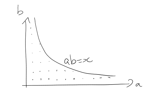
Dirichlet hyperbola method

Problem: How many lattice points $(a, b) \in ℕ^{2}$ satisfy $a b \leq x$ ?

Note that this number is $\sum_{n \leq x} τ (n) = \sum_{a b \leq x} 1$ .

Dirichlet proved that for $x \geq 2$ ,

\sum_{n \leq x} τ (n) = x \log x + (2 γ - 1) x + O (x^{1 ∕ 2})

where $γ$ is Euler’s constant.

We will see a proof of this shortly.

Conjecture: Can have $O_{𝜀} (x^{\frac{1}{4} + 𝜀})$ . Current best exponent is $0.314$ .

First, we prove a lemma:

Lemma (Dirichlet hyperbola method). Assuming that:

$f, g : ℕ \to ℂ$
$x \geq y \geq 1$

Then

\sum_{n \leq x} (f * g) (n) = \sum_{d \leq y} f (d) \sum_{m \leq \frac{x}{d}} g (m) + \sum_{m \leq \frac{x}{y}} g (m) \sum_{y < d \leq \frac{x}{m}} f (d) .

Proof. $\sum_{n \leq x} (f * g) (n) = \sum_{d m \leq x} f (d) g (m)$ . Split this sum into parts with $d \leq y$ and $d > y$ to get the conclusion. □

Theorem 1.5 (Dirichlet’s divisor problem). For $x \geq 2$ ,

\sum_{n \leq x} τ (n) = x \log x + (2 γ - 1) x + O (x^{1 ∕ 2})

where $γ$ is Euler’s constant.

Proof. We use the Dirichlet hyperbola method, with $y = x^{\frac{1}{2}}$ . Note that $τ = 1 * 1$ . Then,

\begin{array}{l} \sum_{n \leq x} τ (n) & = \sum_{d \leq x^{\frac{1}{2}}} \sum_{m \leq \frac{x}{d}} 1 + \sum_{m \leq x^{\frac{1}{2}}} \sum_{x^{\frac{1}{2}} < d \leq \frac{x}{m}} 1 \\ = \sum_{x \leq x^{\frac{1}{2}}} (\frac{x}{d} + O (1)) + \sum_{m \leq x^{\frac{1}{2}}} (\frac{x}{m} - x^{\frac{1}{2}} + O (1)) \\ = x \sum_{d \leq x^{\frac{1}{2}}} \frac{1}{d} + x \sum_{m \leq x^{\frac{1}{2}}} \frac{1}{m} - \sum_{m \leq x^{\frac{1}{2}}} x^{\frac{1}{2}} + O (x^{\frac{1}{2}}) \end{array}

Recall from Lecture 2 that

\sum_{d \leq y} \frac{1}{d} = \log y + γ + O (\frac{1}{y}) .

Taking $y = x^{\frac{1}{2}}$ , the previous expression becomes

2 \times (\frac{1}{2} \log x + γ + O (\frac{1}{x^{\frac{1}{2}}})) - x + O (x^{\frac{1}{2}}) = x \log x + (2 γ - 1) x + O (x^{\frac{1}{2}}) . □

2 Elementary Estimates for Primes

Recall from Lecture 1:

$\sum_{p} \frac{1}{p} = \infty$ (Euler’s Theorem)
$π (x) ≪ \frac{x}{\log x}$ (Chebyshev’s Theorem)

2.1 Merten’s Theorems

Theorem 2.1 (Merten’s Theorem). Assuming that:

$x \geq 3$

Then

(i) $\sum_{p \leq x} \frac{\log p}{p} = \log x + O (1)$
(ii) $\sum_{p \leq x} \frac{1}{p} = \log \log x + M + O (\frac{1}{\log x})$ (for some $M \in ℝ$ )
(iii) $\prod_{p \leq x} (1 - \frac{1}{p}) = \frac{c + o (1)}{\log x}$ (for some $c > 0$ )

Remark. Can show $c = e^{- γ}$ .

Proof.

(i) Let

N = ⌊ x ⌋

. Consider

N!

. We have

\begin{array}{l} N^{N} & \leq N^{N} \\ N! & \geq N^{N} e^{- N} \end{array}

(the second inequality cn be proved by induction, using ${(1 + \frac{1}{N})}^{N} \leq e$ ).

Let $v_{p} (k)$ be the largest power of $p$ dividing $k$ . Then

\begin{array}{l} N! & = \prod_{p \leq N} p^{v_{p} (N!)} & (fundamental theorem of arithmetic) \\ ⟹ \log N! & = \sum_{p \leq N} v_{p} (N!) \log p \end{array}

We have $v_{p} (N!) = \sum_{j = 1}^{\infty} ⌊ \frac{N}{p^{j}} ⌋$ . Indeed,

\begin{array}{l} v_{p} (N!) & = \sum_{k = 1}^{N} v_{p} (k) \\ = \sum_{k = 1}^{N} \sum_{j = 1}^{\infty} 𝟙_{v_{p} (k) \geq j} \\ = \sum_{j = 1}^{\infty} \sum_{k = 1}^{N} 𝟙_{v_{p} (k) \geq j} \\ = \sum_{j = 1}^{\infty} ⌊ \frac{N}{p^{j}} ⌋ \end{array}

Now,

\begin{array}{l} \log N! & = \sum_{p \leq N} ⌊ \frac{N}{p} ⌋ \log p + \sum_{p \leq N} (\log p) \sum_{j = 2}^{\infty} ⌊ \frac{N}{p^{j}} ⌋ \\ = \sum_{p \leq N} (\frac{N}{p} + O (1)) \log p + O (\sum_{p \leq N} \frac{\log p}{p^{2}} \cdot N) & (geometric series) \\ = N \sum_{p \leq N} \frac{\log p}{p} + \underset{\leq (\log N) π (N) ≪ N (C h e b y s h e v)}{\underset{⏟}{O (\sum_{p \leq N} \log p)}} + O (N) & (since \sum_{p} \frac{\log p}{p^{2}} < \infty) \\ = N \sum_{p \leq N} \frac{\log p}{p} + O (N) \end{array}

Combine with $\log N! = N \log N + O (N)$ to get

N \log N + O (N) = N \sum_{p \leq N} \frac{\log p}{p} + O (N) .

Divide by $N$ to get the result.

(ii) By Partial Summation, this is
$1 + O (\frac{1}{\log x}) + \int_{2}^{x} \frac{\sum_{p \leq t} \frac{\log p}{p}}{t {(\log t)}^{2}} d t .$

Writing $𝜀 (t) = \sum_{p \leq t} \frac{\log p}{p} - \log t$ , we get
$\begin{array}{l} 1 + O (\frac{1}{\log x}) + \int_{2}^{x} \frac{d t}{t \log t} + \int_{2}^{x} \frac{𝜀 (t)}{t {(\log t)}^{2}} d t \\ = 1 + O (\frac{1}{\log x}) + \log \log x - \log \log 2 + \int_{2}^{\infty} \frac{𝜀 (t)}{t {(\log t)}^{2}} d t + O (\int_{x}^{\infty} \frac{| 𝜀 (t) |}{t {(\log t)}^{2}} d t) \end{array}$
By part (i),
$\begin{array}{l} \int_{x}^{\infty} \frac{| 𝜀 (t) |}{t {(\log t)}^{2}} d t \\ ≪ \int_{x}^{\infty} \frac{1}{t {(\log t)}^{2}} d t \\ ≪ \frac{1}{\log x} \end{array}$
Take $M = 1 - \log \log 2 + \int_{2}^{\infty} \frac{𝜀 (t)}{t {(\log t)}^{2}} d t$ .
(iii) Use Taylor expansion
$\log (1 - y) = - \sum_{j = 1}^{\infty} \frac{y^{j}}{j}$

to get
$\begin{array}{l} \log \prod_{p \leq x} (1 - \frac{1}{p}) & = \sum_{p \leq x} \log (1 - \frac{1}{p}) \\ = - \sum_{p \leq x} \frac{1}{p} - \sum_{p \leq x} \sum_{j = 2}^{\infty} \frac{p - j}{j} \end{array}$
Write $H = \sum_{p} \sum_{j = 2}^{\infty} \frac{p - j}{j}$ . We get
$\begin{array}{l} = - \sum_{p \leq x} \frac{1}{p} - H + O (\sum_{p > x} \underset{≪ p^{- 2}}{\underset{⏟}{\sum_{j = 2}^{\infty} \frac{p - j}{j}}}) \\ = - \sum_{p \leq x} \frac{1}{p} - H + O (\frac{1}{x}) \\ \overset{(ii)}{=} - \log \log x - H + O (\frac{1}{x}) \end{array}$
Taking exponentials,
$\prod_{p \leq x} (1 - \frac{1}{p}) = \frac{c + o (1)}{\log x} . □$

2.2 Sieve Methods

General tools for estimating the number of primes (or products of a few primes in a set).
Need information on the distribution of the set in residue classes.

Definition (Sieve problem). Let $P \subseteq ℙ$ . Let

P (z) = \prod_{\begin{array}{c} p \in P \\ p \leq z \end{array}} p,

and let $A \subseteq ℤ$ . Denote

S (A, P, z) = | {n \in A : (n, P (z)) = 1} | .

Problem: Estimate $S (A, P, z)$ .

Note that if $A \subseteq [\frac{x}{2}, x] \cap ℤ$ ,

\begin{array}{l} S (A, ℙ, x^{\frac{1}{2}}) & = | A \cap ℙ | \\ S (A, ℙ, x^{\frac{1}{3}}) & = | A \cap (ℙ \cup {p_{1} p_{2} : p_{1} p_{2} > x^{\frac{1}{3}}}) | \end{array}

Sieve hypothesis: There exists a multiplicative $g : ℕ \to [0, 1]$ and $R_{d} \in ℝ$ such that

| {n \in A : n \equiv 0 (m o d d)} | = g (d) | A | + R_{d}

for all square-free $d$ (no repeated prime factors).

Example.

$A = [1, x]$ , $P = ℙ$ .

| A_{d} | = ⌊ \frac{x}{d} ⌋ = \frac{x}{d} + O (1)

Then $g (d) = \frac{1}{d}$ , $| R_{d} | ≪ 1$ .

S (A, ℙ, x^{\frac{1}{2}}) = | {p \in ℙ : p \in [x^{\frac{1}{2}}, x]} | = π (x) + O (x^{\frac{1}{2}}) .

$A = {n (n + 2) : n \leq x}$ , $P = ℙ$ . Let $d = p_{1} \dots p_{r}$ , where $p_{i}$ are distinct primes. Then
$\begin{array}{l} | A_{d} | & = | {n \leq x : n \equiv 0 or - 2 (m o d p_{i}) \forall i \leq r} | \\ = {\begin{matrix} \frac{2^{r}}{d} x & if d odd \\ \frac{2^{r - 1}}{d} x + O (2^{r}) & if d even \end{matrix} \end{array}$
(by Chinese Remainder Theorem).
$\begin{array}{l} S (A, ℙ, {(2 x)}^{\frac{n}{2}}) & = | {p \in ({(2 x)}^{\frac{1}{2}}, x] : p + 2 \in ℙ} | \\ = | {p \leq x : p + 2 \in ℙ} | + O (x^{\frac{1}{2}}) \end{array}$
Here,
$g (p) = {\begin{matrix} \frac{1}{p} & p = 2 \\ \frac{2}{p} & p > 2 \end{matrix}$

and $R_{d} = O (2^{w (d)})$ , where $w (d)$ is the number of prime factors of $d$ (distinct).

Lemma. We have

S (A, P, z) = \sum_{d | P (z)} μ (d) | A_{d} | .

Proof. Recall that

𝟙_{n = 1} = (μ * 1) (n)

(since $μ$ is the inverse of $1$ ). Hence,

\begin{array}{l} S (A, P, z) & = \sum_{n \in A} 𝟙_{(n, P (z)) = 1} \\ = \sum_{n \in A} \sum_{\begin{array}{c} d | P (z) \\ d | n \end{array}} μ (d) \\ = \sum_{d | P (z)} μ (a) | A_{d} | □ \end{array}

Example. Let

π (x, z) = | {n \leq x : (n, P (z)) = 1} | .

Let $P = ℙ$ . Let $A = [1, x] \cap ℤ$ . Then

| A_{d} | = \frac{x}{d} + O (1) .

By the previous lemma,

\begin{array}{l} π (x, z) & = S (A, ℙ, z) \\ = \sum_{d | P (z)} μ (d) (\frac{x}{d} + O (1)) \\ = x \sum_{d | P (z)} \frac{μ (d)}{d} + O (\sum_{d | P (z)} \underset{\leq 1}{\underset{⏟}{| μ (d) |}}) \\ = x \sum_{d | P (z)} \frac{μ (d)}{d} + O (2^{π (z)}) & P (z) = p_{1} \dots p_{π (2)} \\ = x \prod_{p \leq z} (1 + \underset{- 1}{\underset{⏟}{\frac{μ (p)}{p}}}) + O (2^{π (2)}) & fundamental theorem of arithmetic \\ = \frac{c + o (1)}{\log z} x + O (2^{z}) & Merten’s theorem, for some c > 0 \end{array}

For $2 \leq z \leq \log x$ ,

π (x, z) = \frac{c + o (1)}{\log z} x .

Theorem (Sieve of Erastothenes – Legendre). Assuming that:

$A \subseteq [1, x] \cap ℕ$
$2 \leq z \leq x$
Assume the Sieve Hypothesis

Then

\begin{array}{l} S (A, P, z) \\ = | A | \prod_{\begin{array}{c} p \leq 2 \\ p \in P \end{array}} (1 - g (p)) + O (x^{\frac{1}{2}} {(\log x)}^{\frac{1}{2}} 2^{- \frac{\log x}{4 \log z}} {(\sum_{\begin{array}{c} d \leq x \\ d | P (z) \end{array}} | R_{d} |^{2})}^{\frac{1}{2}} + | A | e^{\frac{\log x}{\log z}} \prod_{\begin{array}{c} p \leq z \\ p \in P \end{array}} {(1 + g (p))}^{e}) \end{array}

Proof. Recall from previous lecture that

\begin{array}{l} S (A, P, z) & = \sum_{\begin{array}{c} d | P (z) \\ d \leq x \end{array}} μ (d) | A_{d} | & (since A_{d} = \emptyset for d > x) \\ = \sum_{\begin{array}{c} d | P (z) \\ d \leq x \end{array}} μ (d) g (d) | A | + O (\sum_{\begin{array}{c} d \leq x \\ d | P (z) \end{array}} | R_{d} |) & (sieve hypothesis) \\ = | A | \sum_{d | P (z)} μ (d) g (d) + O (\sum_{\begin{array}{c} d \leq x \\ d | P (z) \end{array}} | R_{d} | + | A | \sum_{\begin{array}{c} d | P (z) \\ d > x \end{array}} g (d)) \\ = | A | \prod_{\begin{array}{c} p \leq z \\ p \in P \end{array}} (1 - g (p)) + O (\sum_{\begin{array}{c} d \leq x \\ d | P (z) \end{array}} | R_{d} | + | A | \sum_{\begin{array}{c} d | P (z) \\ d > x \end{array}} g (d)) \end{array}

We estimate the first error term using Cauchy-Schwarz:

\sum_{\begin{array}{c} d \leq x \\ d | P (z) \end{array}} | R_{d} | \leq {(\sum_{\begin{array}{c} d \leq x \\ d | P (z) \end{array}} | R_{d} |^{2})}^{\frac{1}{2}} {(\sum_{\begin{array}{c} d \leq x \\ d | P (z) \end{array}} 1)}^{\frac{1}{2}} .

Note that if $d | P (z)$ , $d > x^{\frac{1}{2}}$ , then

ω (d) \geq \frac{\log x^{\frac{1}{2}}}{\log z},

( $ω (d)$ – number of distinct prime factors of $d$ ), since $z^{ω (d)} \geq d \geq x^{\frac{1}{2}}$ .

Hence, $2^{ω (d)} \geq 2^{\frac{\log x}{2 \log z}}$ , $d | P (z)$ , $d > x^{\frac{1}{2}}$ .

Now we get

\begin{array}{l} \sum_{\begin{array}{c} d \leq x \\ d | P (z) \end{array}} 1 & \leq 2^{- \frac{\log x}{2 \log z}} \sum_{\begin{array}{c} d \leq x \\ d | P (z) \end{array}} \underset{= τ (d)}{\underset{⏟}{2^{ω (d)}}} \\ \leq 2^{- \frac{\log x}{2 \log z}} \sum_{d \leq x} τ (d) \\ ≪ 2^{- \frac{\log x}{2 \log z}} x \log x \end{array}

(the last step is by Dirichlet’s divisor problem: $\sum_{d \leq x} τ (d) = (1 + o (1)) \cdot x \log x$ ).

Substituting this in, the first error term becomes as desired.

Now we estimate the second error term. We have

\begin{array}{l} \sum_{\begin{array}{c} d | P (z) \\ d > x \end{array}} g (d) & \leq x^{- \frac{1}{\log z}} \sum_{d | P (z)} g (d) d^{\frac{1}{\log z}} & (since d > x in the sum: Rankin’s trick) \\ = x^{- \frac{1}{\log z}} \prod_{\begin{array}{c} p \leq z \\ p \in P \end{array}} (1 + g (p) \underset{\leq z^{\frac{1}{\log z}} = e}{\underset{⏟}{p^{\frac{1}{\log z}}}}) \\ \leq x^{- \frac{1}{\log z}} \prod_{\begin{array}{c} p \leq z \\ p \in P \end{array}} (1 + e g (p)) \\ \leq \underset{= e^{- \frac{\log x}{\log z}}}{\underset{⏟}{x^{- \frac{1}{\log z}}}} \prod_{\begin{array}{c} p \leq z \\ p \in P \end{array}} {(1 + g (p))}^{e} & (1 + e y \leq {(1 + y)}^{e}) \end{array}

Combining the error terms, the claim follows. □

Example. Take $A = [1, x] \cap ℤ$ , $P = ℙ$ . Then $g (d) = \frac{1}{d}$ , $R_{d} = O (1)$ , so the sieve gives us

\begin{array}{l} S (A, P, z) & = π (x, z) \\ = (x + O (1)) \prod_{p \leq z} (1 - \frac{1}{p}) \\ + O (x^{\frac{1}{2}} {(\log x)}^{\frac{1}{2}} 2^{- \frac{\log x}{4 \log z}} x^{\frac{1}{2}} + (x + O (1)) e^{- \frac{\log x}{\log z}} \prod_{p \leq z} {(1 + \frac{1}{p})}^{e}) \end{array}

By Merten’s Theorem,

\begin{array}{l} \prod_{p \leq z} (1 - \frac{1}{p}) & = \frac{C + o (1)}{\log z} \\ \prod_{p \leq z} (1 + \frac{1}{p}) & \leq \prod_{p \leq z} {(1 - \frac{1}{p})}^{- 1} \\ = (\frac{1}{C} + o (1)) \log z \end{array}

Hence,

π (x, z) = \frac{c + o (1)}{\log z} + O (x {(\log x)}^{\frac{1}{2}} 2^{- \frac{\log x}{4 \log z}} + x e^{- \frac{\log x}{\log z}} {(\log z)}^{e}) .

Hence, for $2 \leq z \leq \exp (\frac{\log x}{10 \log \log x})$ ,

π (x, z) = \frac{c + o (1)}{\log z} x .

This asymptotic in fact holds for $z \leq x^{o (1)}$ .

In particular, the Erastothenes-Legendre sieve gives

π (x) \leq π (x, z) + z ≪ \frac{x}{\log x} \log \log x

for $z = \exp (\frac{\log x}{10 \log \log x})$ . Not quite the Chebyshev bound $π (x) ≪ \frac{x}{\log x}$ .

2.3 Selberg Sieve

	asymptotes	good upper bound for primes

Erastothenes-Legendre	✓	✗

Selberg	✗	✓

Theorem 2.2 (Selberg sieve). Assuming that:

$z \geq 2$
$A \subseteq ℤ$ finite
$P \subseteq ℙ$
Assume the sieve hypothesis
$h : ℕ \to [0, \infty)$ be the multiplicative function supported on square-free numbers, given on the primes by

$h (p) = {\begin{matrix} \frac{g (p)}{1 - g (p)} & p \in P \\ 0 & p \notin P \end{matrix}$

Then

S (A, P, z) \leq \frac{| A |}{\sum_{d \leq z} h (d)} + \sum_{\begin{array}{c} d \leq z^{2} \\ d | P (z) \end{array}} τ_{3} (d) | R_{d} | .

Sieve hypothesis: There is a multiplicative $g : ℕ \to [0, 1]$ and $R_{d} \in ℝ$ such that

| A_{d} | = g (d) | A | + R_{d}

for all square-free $d \geq 1$ .

Proof. Let ${(ρ_{d})}_{d \in ℕ}$ be real numbers with

ρ_{1} = 1, ρ_{d} = 0, d > z (∗)

Then,

𝟙_{(n, P (z)) = 1} \leq {(\sum_{\begin{array}{c} d | n \\ d | P (z) \end{array}} ρ_{d})}^{2} .

(If $(n, P (z)) = 1$ , get $1 \leq ρ$ otherwise use $0 \leq x^{2}$ ).

Summing over $n \in A$ ,

\begin{array}{l} S (A, P, z) & = \sum_{n \in A} 𝟙_{(n, P (z)) = 1} \\ \leq \sum_{n \in A} {(\sum_{\begin{array}{c} d | n \\ d | P (z) \end{array}} ρ_{d})}^{2} \\ = \sum_{d_{1} d_{2} | P (z)} ρ_{d_{1}} ρ_{d_{2}} \sum_{\begin{array}{c} n \in A \\ [d_{1}, d_{2}] | n \end{array}} 1 \\ = | A | \sum_{d_{1}, d_{2} | P (z)} ρ_{d_{1}} ρ_{d_{2}} g ([d_{1}, d_{2}]) + \underset{E}{\underset{⏟}{\sum_{d_{1}, d_{2} | P (z)} ρ_{d_{1}} ρ_{d_{2}} R_{[d_{1}, d_{2}]}}} & (sieve hypothesis) \end{array}

( $[m, n]$ means $lcm (m, n)$ ).

We first estimate $E$ :

\begin{array}{l} E & \leq \max_{k} | ρ_{k} |^{2} \sum_{d_{1}, d_{2} | P (z)} | R_{[d_{1}, d_{2}]} | \\ = \max_{k} | ρ_{k} |^{2} \sum_{\begin{array}{c} d \leq z^{k} \\ d | P (z) \end{array}} \sum_{\begin{array}{c} d_{1}, d_{2} \in ℕ \\ [d_{1}, d_{2}] = d \end{array}} | R_{d} | & (d = [d_{1}, d_{2}]) \end{array}

We have

\begin{array}{l} \sum_{\begin{array}{c} d_{1}, d_{2} \in ℕ \\ d = [d_{1}, d_{2}] \end{array}} 1 & = \sum_{l \leq z} \sum_{\begin{array}{c} d_{1}^{'}, d_{2}^{'} \in ℕ \\ d = l d_{1}^{'} d_{2}^{'} \\ (d_{1}^{'}, d_{2}^{'}) = 1 \end{array}} 1 & (l = (d_{1}, d_{2}), d_{1}^{'} = d_{1} ∕ l, [d_{1}, d_{2}] = l d_{1}^{'} d_{2}^{'}) \\ \leq τ_{3} (d) \end{array}

Therefore

E \leq \sum_{\begin{array}{c} d \leq z^{z} \\ d | P (z) \end{array}} τ_{3} (d) | R_{d} | \cdot \max_{k} | ρ_{k} |^{2} .

Now it suffices to prove that there is a choice of ${(ρ_{d})}_{d \in ℕ}$ satisfying ( $*$ ) such that

Claim 1: $\sum_{d_{1}, d_{2} | P (z)} ρ_{d_{1}} ρ_{d_{2}} g ([d_{1}, d_{2}]) = \frac{1}{\sum_{d \leq z}} h (d)$ .

Claim 2: $| ρ_{k} | \leq 1$ for all $k \in ℕ$ .

Proof of claim 1:

We have, writing $k = (d_{1}, d_{2})$ , $d_{i}^{'} = \frac{d_{i}}{k}$ ,

\begin{array}{l} \sum_{d_{1}, d_{2} | P (z)} ρ_{d_{1}} ρ_{d_{2}} g ([d_{1}, d_{2}]) & = \sum_{k | P (z)} μ {(k)}^{2} \sum_{\begin{array}{c} d_{1}^{'}, d_{2}^{'} | \frac{P (z)}{k} \\ (d_{1}^{'}, d_{2}^{'}) = 1 \end{array}} ρ_{k d_{1}^{'}} ρ_{k d_{2}^{'}} g (k d_{1}^{'} d_{2}^{'}) \\ = \sum_{k | P (z)} μ {(k)}^{2} g (k) \sum_{\begin{array}{c} d_{1}^{'}, d_{2}^{'} | \frac{P (z)}{k} \\ (d_{1}^{'}, d_{2}^{'}) = 1 \end{array}} ρ_{k d_{1}^{'}} ρ_{k d_{2}^{'}} g (d_{1}^{'}) g (d_{2}^{'}) & (multiplicativity) \end{array}

We have

𝟙_{(d_{1}^{'}, d_{2}^{'}) = 1} = \sum_{\begin{array}{c} c | d_{1}^{'} \\ c | d_{2}^{'} \end{array}} μ (c)

(since $μ * 1 = I$ ) so the previous expression becomes

\begin{array}{l} \sum_{k | P (z)} μ {(k)}^{2} g (k) \sum_{c | \frac{P (z)}{k}} μ (c) \sum_{\begin{array}{c} d_{1}^{'}, d_{2}^{'} | P (z) \\ d_{1}^{'} \equiv 0 (mod () c) \\ d_{2}^{'} \equiv 0 (mod c) \end{array}} ρ_{k d_{1}^{'}} ρ_{k d_{2}^{'}} g (d_{1}^{'}) g (d_{2}^{'}) \\ = \sum_{k | P (z)} μ {(k)}^{2} g (k) \sum_{c | \frac{P (z)}{k}} μ (k) {(\sum_{\begin{array}{c} d | \frac{P (z)}{k} \\ d \equiv 0 (mod c) \end{array}})}^{2} \\ = \sum_{k | P (z)} μ {(k)}^{2} g {(k)}^{- 1} \sum_{c | \frac{P (z)}{k}} μ (c) {(\sum_{d^{'} | \frac{P (z)}{c k}} ρ_{c k d^{'}} g (c k d^{'}))}^{2} \\ = \sum_{n \leq z} h {(m)}^{- 1} {(\sum_{\begin{array}{c} d | P (z) \\ d \equiv 0 (mod n) \end{array}} ρ_{d} g (d))}^{2} \end{array}

(multiplicativity, $d = c d^{'}$ , $m = c k$ , $d = m d^{'}$ ) since $\frac{1}{h} = \frac{μ^{2}}{g} * μ$ (check on primes $\frac{1}{h (p)} = \frac{1}{g (p)} - 1$ ).

Now we get

\sum_{d_{1}, d_{2} | P (z)} ρ_{d_{1}} ρ_{d_{2}} g ([d_{1}, d_{2}]) = \sum_{m \leq z} h {(m)}^{- 1} ζ_{m}^{2}

where

ζ_{m} = \sum_{\begin{array}{c} d | P (z) \\ d \equiv 0 (mod m) \end{array}} ρ_{d} g (d) .

Want to minimise this subject to ( $*$ ).

We need to translate the condition $ρ_{1} = 1$ . Note that

\begin{array}{l} \sum_{\begin{array}{c} m \leq z \\ m \equiv 0 (mod c) \end{array}} μ (m) ζ_{m} & = \sum_{d | P (z)} ρ_{d} g (d) \underset{\sum_{m^{'} | \frac{d}{c}} μ (c) μ (m^{'}) = μ (d) 𝟙_{d = e}}{\underset{⏟}{\sum_{\begin{array}{c} m | d \\ c | m \end{array}} μ (m)}} \\ = μ (e) ρ_{e} g (e) \end{array}

Hence,

ρ_{e} = \frac{μ (e)}{g (e)} \sum_{\begin{array}{c} m \leq 2 \\ m \equiv 0 (mod c) \end{array}} μ (m) ζ_{m} .

Now,

ρ_{1} = 1 = \sum_{m \leq z} μ (m) ζ_{m} .

By Cauchy-Schwarz, we then get

(\sum_{m \leq z} h {(m)}^{- 1} ζ_{m}^{2}) (\sum_{m \leq z} μ {(m)}^{2} h (m)) \geq {(\sum_{m \leq z} μ (m) ζ_{m})}^{2} = 1 .

Hence

\sum_{m \leq z} h {(m)}^{- 1} ζ_{m}^{2} \geq \frac{1}{\sum_{m \leq z} μ {(m)}^{2} h (m)} = \frac{1}{\sum_{m \leq z} h (m)} .

Equality holds for $T_{m} = \frac{h (m)}{G (z)}$ , where $G (z) = \sum_{m \leq z} h (m)$ . We now check that with these $ζ_{m}$ , $ρ_{d} = 0$ for $d > z$ .

Note that

ρ_{c} = \frac{μ (c)}{g (c) G (z)} \sum_{\begin{array}{c} m \leq z \\ m \equiv (mod c) \end{array}} μ (m) h (m) .

Hence, $ρ_{c} = 0$ for $c > 2$ .

This proves Claim 1.

Now we prove Claim 2 ( $| ρ_{c} | \leq 1$ ).

Note that any $m$ has at most one representation as $m = e m^{'}$ , where $e | d$ , $(m^{'}, d) = 1$ (for any $d \in ℕ$ ).

Now,

\begin{array}{l} G (z) & \geq \sum_{c | d} \sum_{\begin{array}{c} m^{'} \leq \frac{z}{c} \\ (m^{'}, d) = 1 \end{array}} h (c m^{'}) \\ = \sum_{c | d} h (c) \sum_{\begin{array}{c} m^{'} \leq \frac{z}{c} \\ (m^{'}, d) = 1 \end{array}} h (m^{'}) \\ \geq \sum_{c | d} h (e) \sum_{\begin{array}{c} m^{'} \leq \frac{z}{d} \\ (m^{'}, d) = 1 \end{array}} h (m^{'}) \end{array}

Now,

ρ_{d} = \frac{μ {(d)}^{2} h (d)}{g (d) G (z)} \sum_{\begin{array}{c} m^{'} \leq \frac{z}{d} \\ (m^{'}, d) = 1 \end{array}} μ (m^{'}) h (m^{'}) .

Substituting the lower bound for $G (z)$ ,

| ρ_{d} | \leq \frac{h (d)}{g (d) \sum_{c | d} h (e)} = 1,

since $1 * h = \frac{h}{g}$ . □

Lemma 2.3. Assuming that:

$z \geq 3$
$g : ℕ \to [0, 1]$ multiplicative

for some

K, A \in ℝ

we have

\sum_{p \leq z} g (p) \log p \leq κ \log z + A .

Then

\frac{1}{\sum_{m \leq z} h (m)} \leq 2 \prod_{p \leq z^{1 ∕ (e κ + 1)}} (1 - g (p)),

where $h$ is defined in terms of $g$ as in Selberg’s sieve.

Proof. Note that for any $c \in (0, 1)$ ,

\sum_{m \leq z} h (m) \geq \sum_{\begin{array}{c} m \leq z \\ m | P (z^{c}) \end{array}} h (m) = G (z, c) .

Then

\begin{array}{l} \prod_{\begin{array}{c} p \leq z^{c} \\ p \in P \end{array}} {(1 - g (p))}^{- 1} - G (z, c) & = \prod_{\begin{array}{c} p \leq z^{c} \\ p \in P \end{array}} (1 + h (p)) - \sum_{\begin{array}{c} m \leq z \\ m | P (z^{c}) \end{array}} h (m) \\ = \sum_{\begin{array}{c} m > z \\ m | P (z^{c}) \end{array}} h (m) \end{array}

By Rankin’s trick,

\begin{array}{l} 1 - \prod_{p \leq z^{c}} (1 - g (p)) G (z, c) & = \prod_{p \leq z^{c}} (1 - g (p)) \sum_{\begin{array}{c} m > z \\ m | P (z^{c}) \end{array}} h (m) \\ \leq \prod_{p \leq z^{c}} (1 - g (p)) z^{- \frac{λ}{\log z}} \sum_{m | P (z^{c})} h (m) m^{\frac{λ}{\log z}} & (for any λ > 0) \\ = \prod_{p \leq z^{c}} (1 - g (p)) e^{- λ} \prod_{p \leq z^{c}} (1 + h (p) p^{\frac{λ}{\log z}}) \\ = e^{- λ} \prod_{p \leq z^{c}} (1 - g (p) + g (p) p^{\frac{λ}{\log z}} \\ \leq e^{- λ} \exp (\sum_{p \leq z^{c}} \underset{\leq \frac{λ}{\log z} (\log p) p^{\frac{λ}{\log z}}}{\underset{⏟}{(p^{\frac{λ}{\log z}} - 1)}}) \\ \leq \exp (- λ + \frac{λ}{\log z} \sum_{p \leq z^{c}} g (p) (\log p) p^{\frac{λ}{\log z}}) & (1 + t \leq e^{t}) \\ \leq \exp (- λ + c e^{c λ} λ κ + λ e^{c λ} \frac{A}{\log z}) \end{array}

Choose $c = \frac{1}{λ}$ and $λ = e κ + 1$ to get the claim. □

The Brun-Titchmarsh Theorem

Theorem 2.4 (Brun-Titchmarsh Theorem). Assuming that:

$x \geq 0$ , $y \geq 2$
$𝜀 > 0$ and $y$ is large in terms of $𝜀$

Then

π (x + y) - π (x) \leq \frac{(2 + 𝜀) y}{\log y} .

Remark. We expect

π (x + y) - π (x) = \frac{(n + o (1)) y}{\log x}

in a wide range of $y$ (e.g. $y \geq x^{𝜀}$ for some $𝜀 > 0$ fixed). The prime number theorem gives this for $y ≫ x$ . The Brun-Titchmarsh Theorem gives an upper bound of the expected order for $y \geq x^{𝜀}$ .

Proof. Apply the Selberg sieve with $A = [x, x + y] \cap ℕ$ , $P = ℙ$ . Note that for any $d \geq 1$ ,

| {a \in A : a \equiv 0 (m o d d)} = \frac{y}{d} + O (1) .

Hence, the sieve hypothesis holds with $g (d) = \frac{1}{d}$ , $R_{d} = O (1)$ .

Now, the function $h$ in Selberg sieve is given on primes by

h (p) = \frac{g (p)}{1 - g (p)} = \frac{1}{p - 1} = \frac{1}{φ (p)},

where $φ$ is the Euler totient function. In general,

h (d) = μ {(d)}^{2} \cdot \frac{1}{φ (d)}

(since $φ$ is multiplicative). Now, for any $z \geq 2$ , Selberg sieve yields

S (A, ℙ, z) \leq \frac{y}{\sum_{d \leq z} \frac{μ {(d)}^{2}}{φ (d)}} + O (\sum_{d \leq z^{2}} τ_{3} (d)) .

By Problem 11 on Example Sheet 1, the error term is $O (z^{2} {(\log z)}^{2})$ .

Take $z = y^{\frac{1}{2} - \frac{𝜀}{10}}$ . Then

z^{2} {(\log z)}^{2} ≪ {(y^{\frac{1}{2} - \frac{𝜀}{10}})}^{2} {(\log y)}^{2} ≪ y^{1 - \frac{𝜀}{20}}

(for $y \geq y_{0} (𝜀)$ ). We estimate

\begin{array}{l} \sum_{d \leq z} \frac{μ {(d)}^{2}}{φ (d)} & = \sum_{d \leq z} \frac{μ {(d)}^{2}}{d} \frac{d}{φ (d)} \\ = \sum_{d \leq z} \frac{μ {(d)}^{2}}{d} \cdot \prod_{p | d} \underset{= \frac{p}{p - 1} = \frac{p}{φ (p)}}{\underset{⏟}{(1 + \frac{1}{p} + \frac{1}{p^{2}} + \dots)}} \\ \geq \sum_{n \leq z} \frac{1}{n} \end{array}

since any $n \leq z$ has at least one representation as

n = d p_{1}^{a_{1}} \dots p_{k}^{a_{k}},

where $d \leq z$ is square-free and $p_{i} | d$ are primes and $a_{1} \geq 0$ .

We have proved

\sum_{n \leq z} \frac{1}{n} = \log z + O (1) \geq (1 - \frac{1}{10}) \log z

for $z \geq z_{0} (𝜀)$ .

Putting everything together gives us

\begin{array}{l} π (x + y) - π (x) & \leq S (A, ℙ, z) + z \\ \leq \frac{y}{(1 - \frac{𝜀}{10}) \log z} + z + y^{1 - \frac{𝜀}{20}} \\ \leq \frac{(2 + 𝜀) y}{\log y} \end{array}

for $y \geq y_{0} (𝜀)$ . □

3 The Riemann Zeta Function

Recall that the Riemann zeta function is defined by

ζ (s) = \sum_{n = 1}^{\infty} \frac{1}{n^{s}}

for $Re (s) > 1$ .

Remarkable properties:

(1) $ζ (s)$ extends meromorphically to $ℂ$ .
(2) A functional equation relating $ζ (s) \leftrightarrow ζ (1 - s)$ .
(3) All the (non-trivial) zeroes appear to be on the line $Re (s) = \frac{1}{2}$ (Riemann hypothesis).
(4) $ζ (s)$ closely relates to the distribution of primes.

Notation. $f (x) ≍ g (x)$ means $f (x) ≪ g (x) ≪ f (x)$ . $≍_{σ}$ means that the constant in $≪$ can depend on $σ$ .

Lemma 3.1. Assuming that:

$σ > 1$
$t \in ℝ$

Then

| ζ (σ + i t) | ≍_{σ} 1

Proof. By the Euler product formula,

ζ (σ + i t) = \prod_{p} {(1 - p^{- σ - i t})}^{- 1},

hence

| ζ (σ + i t) | = \prod_{p} | 1 - p^{- σ - i t} |^{- 1} .

By the triangle inequality,

1 - p^{- σ} \leq | 1 - p^{- σ - i t} | \leq 1 + | p^{- σ - i t} | = 1 + p^{- σ} .

Hence,

\prod_{p} {(1 - p^{- σ})}^{- 1} \geq | ζ (σ + i t) | \geq \prod_{p} {(1 = p^{- σ})}^{- 1} .

Note that these products converge if and only if $\sum_{p} p^{- σ}$ converges, and this sum converges by the comparison test. □

Lemma 3.2 (Polynomial growth of $e t a$ in half-planes).

(i)
$f (ζ)$ extends to a meromorphic function on $ℂ$ , with the only pole being a simple pole which is at $s = 1$ .
(ii)
Let $k \geq 0$ be an integer. Then, for $Re (s) \geq - k$ and $| s - 1 | \geq \frac{1}{10}$ we have $| ζ (s) | ≪_{k} | s |^{k + 2} + 1$ .

Proof. Let $k \geq 0$ be an integer.

We claim that there exist polynomials $P_{k}$ , $Q_{k}$ of degree $\leq k + 1$ and such that for $Re (s) > 1$ ,

ζ (s) = \frac{1}{s - 1} + Q_{k} (s) + s (s + 1) \dots (s + k) \int_{1}^{\infty} \frac{P_{k} ({t})}{t^{s + k + 1}} d t . (∗)

First assume ( $*$ ) holds.

Then, since $P_{k} ({t}) ≪_{k} 1$ , for $Re (s) > - k - \frac{1}{2}$ , $| s - 1 | \geq \frac{1}{10}$ , ( $*$ ) gives $| ζ (s) | ≪_{k} | s |^{k + 2} + 1$ . So (ii) follows.

For (i), using analytic continuation and ( $*$ ), it suffices to show that the RHS of ( $*$ ) is meromorphic for $Re (s) > - k$ , with the only pole a simple one at $s = 1$ .

Suffices to show that

\int_{1}^{\infty} \frac{P_{k} ({t})}{t^{s + k + 1}} d t

is analytic for $Re (s) > - k$ .

This follows from the following criterion: If $U \subseteq ℂ$ is open, $f : U \times ℝ \to ℂ$ is piecewise continuous, and if $s \mapsto f (s, t)$ is analytic in $U$ for any $t \in ℝ$ , then $\int_{ℝ} f (s, t) d t$ is analytic in $U$ , provided that $\int_{ℝ} | f (s, t) | d t$ is bounded on compact subsets of $U$ .

Applying this with $f (s, t) = \frac{P_{k} ({t})}{t^{s + k + 1}} 𝟙_{[1, \infty)}$ concludes the proof of (i) assuming ( $*$ ).

We are left with proving ( $*$ ). We use induction on $k$ .

Case $k = 0$ : By Partial Summation,

\begin{array}{l} ζ (s) & = \sum_{n = 1}^{\infty} \frac{1}{n^{s}} \\ = s \int_{1}^{\infty} \frac{⌊ u ⌋}{u^{s + 1}} d u & (apply partial summation to \sum_{n \leq x} n^{- s} and let x \to \infty) \\ = s \int_{1}^{\infty} \frac{1}{u^{s}} d u - \int_{1}^{\infty} \frac{{u}}{u^{s + 1}} d u \\ = \frac{1}{s - 1} + 1 - s \int_{1}^{\infty} \frac{{u}}{u^{s + 1}} d u \end{array}

Take $P_{0} (u) = u$ , $Q_{0} (u) = 1$ .

Case $k + 1$ assuming $k$ : Let

c_{k} = \int_{0}^{1} P_{k} ({t}) d t .

For $Re (s) > 1$ , we have

ζ (s) = \frac{1}{s - 1} + Q_{k} (s) + c_{k} s (s + 1) \dots (s + k - 1) + s (s + 1) \dots (s + k) \int_{1}^{\infty} \frac{P_{k} ({t}) - c_{k}}{t^{s + k + 1}} d t .

Let

P_{k + 1} (u) = - \int_{0}^{u} (P_{k} (t) - c_{k}) d t .

This is a polynomial of degree $\leq k + 2$ . By integration by parts,

\int_{1}^{\infty} \frac{P_{t} ({t}) - c_{k}}{t^{s + k + 1}} d t = (s + k + 1) \int_{1}^{\infty} \frac{P_{k + 1} ({u})}{u^{s + k + 1}} d u .

Substituting this into the previous equation, we get that case $k + 1$ follows. □

The Gamma function

Definition (Gamma function). For $Re (s) > 0$ , let

Γ (s) = \int_{0}^{\infty} t^{s - 1} e^{- t} d t .

Lemma 3.3. $Γ (s)$ is analytic for $Re (s) > 0$ .

Proof. Apply the same criterion for integral of analytic function being analytic as in the previous lemma, taking $f (s, t) = t^{s - 1} e^{- t} 𝟙_{[0, \infty)} (t)$ .

Note that for $0 < σ_{1} \leq Re (s) \leq σ_{2}$ ,

\int_{ℝ} | f (s, t) | d t \leq \int_{0}^{1} t^{σ_{1} - 1} e^{- t} d t + \int_{1}^{\infty} t^{σ_{2} - 1} e^{- t} d t < \infty . □

Lemma (Functional equation for $Γ$ ). The $Γ$ function extends meromorphically to $ℂ$ , with the only poles being simple poles at $s = 0, - 1, - 2, \dots$ .

Moreover:

(i) $Γ (s + 1) = s Γ (s)$ for $s \in ℂ$ .
(ii) $Γ (s) Γ (1 - s) = \frac{π}{\sin (π s)}$ for all $s \in ℂ$ (Euler reflection formula).

Proof.

(i) For

Re (s) > 0

, by integration by parts,

\int_{0}^{\infty} t^{s} e^{- t} d t = s \int_{0}^{\infty} t^{s - 1} e^{- t} d t .

This proves (i) for $Re (s) > 0$ .

Now for any $k \in ℕ$ , for $Re (s) > 0$ we have

Γ (s) = \frac{Γ (s + k)}{(s + k - 1) \dots (s + 1) s} .

The RHS is analytic for $Re (s) > - k$ , so can use analytic continuation to extend $Γ (s)$ meromorphically to $Re (s) > - k$ , with the only poles being simple poles at $s = 0, - 1, \dots, - k, - 1$ .

Let $k \to \infty$ .

(ii) Since both sides are analytic in $ℂ ∖ ℤ$ , by analytic continuation, it suffices to prove the formula for $0 < s < 1$ .
Now, for any $t > 0$ ,
$\begin{array}{l} t^{s - 1} Γ (s - 1) & = t^{s - 1} \int_{0}^{\infty} u^{- s} e^{- u} d u \\ = \int_{0}^{\infty} v^{- s} e^{- v t} d t & (u = v t) \end{array}$
Multiply by $e^{- t}$ and integrate, and use Fubini to get
$\begin{array}{l} Γ (s) Γ (s - 1) & = \int_{0}^{\infty} \int_{0}^{\infty} v^{- s} e^{- v t} d v e^{- t} d t \\ = \int_{0}^{\infty} \int_{0}^{\infty} e^{- (v + 1) t} d t v^{- s} d v \\ = \int_{0}^{\infty} \frac{v^{- s}}{1 + v} d v \\ = \int_{- \infty}^{\infty} \frac{e^{(1 - s) x}}{1 + e^{x}} d x & (v = e^{x}) \end{array}$
Hence, the remaining task is to show
$\int_{- \infty}^{\infty} \frac{e^{(1 - s) x}}{1 + e^{x}} d x = \frac{π}{\sin (π s)} .$

We will do this next time.

□

Theorem 3.4 (Functional equation for $z e t a$ ). Assuming that:

$ξ (s) = \frac{1}{2} s (s - 1) π^{- s ∕ 2} Γ (\frac{s}{s}) ζ (s)$ for $s \in ℂ$

Then

ξ

is an entire function and

ξ (s) = ξ (1 - s)

for

s \in ℂ

. Hence

π^{- s ∕ 2} Γ (\frac{s}{2}) ζ (s) = π^{- \frac{1 - s}{2}} Γ (\frac{1 - s}{2}) ζ (1 - s)

for $s \in ℂ ∖ {0, 1}$ .

Proof. Let $Re (s) > 1$ . Then,

Γ (\frac{s}{2}) = \int_{0}^{\infty} t^{\frac{s}{2} - 1} e^{- t} d t .

Make the change of variables $f = π n^{2} u$ to get

Γ (\frac{s}{2}) = π^{s ∕ 2} n^{s} \int_{0}^{\infty} u^{\frac{s}{2} - 1} e^{- π n^{2} u} d u .

Hence

π^{- \frac{s}{2}} n^{- s} Γ (\frac{s}{2}) = \int_{0}^{\infty} u^{\frac{s}{2} - 1} e^{- π n^{2} u} d u .

Summing over $n \in ℕ$ and using Fubini,

\begin{array}{l} π^{- \frac{s}{2}} Γ (\frac{s}{2}) ζ (s) & = \sum_{n = 1}^{\infty} \int_{0}^{\infty} u^{\frac{s}{2} - 1} e^{- π n^{2} u} d u \\ = \frac{1}{2} \int_{0}^{\infty} u^{\frac{s}{2} - 1} (𝜃 (u) - 1) d u & 𝜃 (u) = \sum_{n = - \infty}^{\infty} e^{- π n^{2} u} \\ = \frac{1}{2} \int_{0}^{1} u^{\frac{s}{2} - 1} (𝜃 (u) - 1) d u + \frac{1}{2} \int_{1}^{\infty} u^{\frac{s}{2} - 1} (𝜃 (u) - 1) d u & (*) \end{array}

By the functional equation

𝜃 (u) = \frac{1}{\sqrt{u}} 𝜃 (\frac{1}{u}),

we have

\begin{array}{l} \int_{0}^{1} u^{\frac{s}{2} - 1} (𝜃 (u) - 1) d u & = \int_{0}^{1} u^{\frac{s}{2} - \frac{3}{2}} 𝜃 (\frac{1}{u}) d u - \int_{0}^{1} u^{\frac{s}{2} - 1} d u \\ = \int_{1}^{\infty} v^{- \frac{s + 1}{2}} 𝜃 (v) d v - \int_{0}^{1} u^{\frac{s}{2} - 1} d u & (u = \frac{1}{v}) \\ = \int_{1}^{\infty} v^{- \frac{s + 1}{2}} (𝜃 (v) - 1) d v + \underset{\frac{1}{\frac{s - 1}{2}}}{\underset{⏟}{\int_{1}^{\infty} v^{- \frac{s + 1}{2}} d v}} - \underset{\frac{1}{\frac{s}{2}}}{\underset{⏟}{\int_{0}^{1} u^{\frac{s}{2} - 1} d u}} \end{array}

Plugging this into ( $*$ ), we get

π^{- \frac{s}{2}} Γ (\frac{s}{2}) ζ (s) = \frac{1}{2} \int_{1}^{\infty} (u^{- \frac{s + 1}{2}} + u^{\frac{s}{2} - 1}) (𝜃 (u) - 1) d u - \frac{1}{s (s - 1)} .

Hence

ξ (s) = - \frac{1}{2} + \frac{1}{4} s (s - 1) \int_{1}^{\infty} (u^{- \frac{s + 1}{2}} + u^{\frac{s}{2} - 1}) (𝜃 (u) - 1) d u . (∗∗)

Since $| 𝜃 (u) - 1 | ≪ e^{- π u}$ , applying the criterion for integrals of analytic functions being analytic, we see that $ξ (s)$ is entire. So by analytic continuation, ( $* *$ ) holds for all $s \in ℂ$ .

Moreover, the expression for $ζ (s)$ is symmetric with respect to $s \mapsto 1 - s$ , so $ξ (s) = ξ (1 - s)$ , $s \in ℂ$ . □

Corollary 3.5 (Zeroes and poles of $z e t a$ ). The $ζ$ function extends to a meromorphic function in $ℂ$ and it has

(i)
Only one pole, which is a simple pole at $s = 1$ , residue $1$ .
(ii)
Simple zeroes at $s = - 2, - 4, - 6, \dots$ .
(iii)
Any other zeroes satisfy $0 \leq Re (s) \leq 1$ .

Proof.

(ii) – (iii) Follows from the lemma on polynomial growth of $ζ$ on vertical lines.
(ii) – (iii) We know $ζ (s) \neq 0$ for $Re (s) > 1$ . We want to show that if $ζ (s) = 0$ and $Re (s) > 0$ then $s \in {- 2, - 4, - 6, \dots}$ and $s$ is a simple zero.
Let $Re (s) > 0$ . By the functional equation for $ζ$ ,

$ζ (s) = \underset{\neq 0}{\underset{⏟}{π^{s - \frac{1}{2}}}} \frac{Γ (\frac{1 - s}{2})}{Γ (\frac{s}{2})} ζ (1 - s) .$

We claim that $Γ (s) \neq 0$ for all $s \in ℂ$ . By the Euler reflection formula,
$Γ (s) Γ (1 - s) \sin (π s) = π,$

for $s \in ℂ$ .

If $Γ (s) = 0$ , then $Γ$ has a pole at $1 - s$ . Hence, $1 - s = - n$ for some $n \geq 0$ integer. But then $s = n + 1$ , and $Γ (n + 1) = n! \neq 0$ .

We conclude that for $Re (s) < 0$ ,
$\begin{array}{l} ζ (s) = 0 & ⟺ \frac{s}{2} is a pole of Γ \\ ⟺ s = - 2 n, n \in ℕ \end{array}$
Since the poles of $Γ$ are simple, $ζ$ has a simple zero at $s = - 2 n$ , $n \in ℕ$ . □

3.1 Partial fraction approximation of $ζ$

This is a formula for $\frac{ζ^{'} (s)}{ζ (s)}$ .

For the proof we need a lemma. We write, for $z \in ℂ$ , $r > 0$ ,

\begin{array}{l} B (z_{0}, r) & = {z \in ℂ : | z - z_{0} | < r} \\ \bar{B (z_{0}, r)} & = {z \in ℂ : | z - z_{0} | \leq r} \\ \partial B (z_{0}, r) & = {z \in ℂ : | z - z_{0} | = r} \end{array}

Lemma 3.6 (Borel-Caratheodory Theorem). Assuming that:

$0 < r < R$
$f$ analytic in $\bar{B (0, R)}$ , with $f (0) = 0$

Then

\sup_{| z | \leq r} | f (z) | \leq \frac{2 r}{R - r} \sup_{| z | = R} Re (f (z)) .

Proof. This is Exercise 10 on Example Sheet 2. □

Lemma 3.7 (Landau). Assuming that:

$z_{0} \in ℂ$ and $r > 0$
$f$ analytic in $B (z_{0}, r)$
for some $M > 1$ we have $| f (z) | < e^{M} | f (z_{0}) |$ for all $z \in B (z_{0}, r)$

Then for

z \in B (z_{0}, r ∕ 4)

| \frac{f^{'} (z)}{f (z)} - \sum_{ρ \in Z} \frac{1}{z - ρ} | \leq \frac{96 M}{r},

where $Z$ is the set of zeroes of $f$ in $\bar{B (z_{0}, r ∕ 2)}$ , counted with multiplicities.

Note. If $f$ is a polynomial, we can factorise

f (z) = a \prod_{ρ} (z - ρ),

and then

\begin{array}{l} \frac{f^{'} (z)}{f (z)} & = {(\log f (z))}^{'} \\ = {(\log a + \sum_{ρ} \log (z - ρ))}^{'} \\ = \sum_{ρ} \frac{1}{z - ρ} \end{array}

Proof. Let

g (z) = \frac{f (z)}{\prod_{ρ \in Z} (z - ρ)} .

Then $g$ is analytic and non-vanishing in $\bar{B (z_{0}, r ∕ 2)}$ . Note that

\frac{g^{'} (z)}{g (z)} = \frac{f^{'} (z)}{f (z)} - \sum_{ρ \in Z} \frac{1}{z - ρ}

( $\frac{{(f_{1} - f_{n})}^{'}}{f_{1} - f_{n}} = \sum_{i = 1}^{n} \frac{f_{1}^{'}}{f_{1}}$ ).

Hence, it suffices to prove

| \frac{g^{'} (z)}{g (z)} | \leq \frac{96 M}{r}

for $z \in B (z_{0}, r ∕ 4)$ . Write

h (z) = \frac{g (z_{0} + z)}{g (z_{0})} .

Then $h$ is analytic and non-vanishing in $\bar{B (0, r ∕ 2)}$ , and $h (0) = 1$ . We want to show

| \frac{h^{'} (z)}{h (z)} | \leq \frac{96 M}{r}

for $z \in B (0, r ∕ 4)$ .

For all $z_{0} \in \partial B (0, r)$ we have

| h (z) | = | \frac{f (z_{0} + z)}{f (z_{0})} \prod_{ρ \in Z} \frac{z_{0} - ρ}{z_{0} + z - ρ} | \leq | \frac{f (z_{0} + z)}{f (z_{0})} | < e^{M}

since

| z_{0} - ρ | \leq \frac{r}{2} = r - \frac{r}{2} \leq | z_{0} + z - ρ |

for $z \in \partial B (0, r)$ .

By the maximum modulus principle, $| h (z) | < e^{M}$ for $z \in \bar{B (0, r ∕ 2)}$ , so

Re \log h (z) = \log | h (z) | < M .

By the Borel-Caratheodory Theorem with radii $\frac{3 r}{8}$ , $\frac{r}{4}$ we have for for $z \in B (0, 3 r ∕ 8)$ ,

| \log h (z) | \leq \frac{2 \frac{r}{4}}{\frac{3 r}{8} - \frac{r}{4}} M = 4 M .

Now, for $z \in B (0, r ∕ 4)$ , Cauchy’s theorem gives us

\begin{array}{l} | \frac{h^{'} (z)}{h (z)} | & = | \frac{1}{2 π i} \int_{\partial B (0, 3 r ∕ 8)} \frac{\log h (w)}{{(z - w)}^{2}} d w | \\ \leq \frac{1}{2 π} \cdot 2 π \frac{3 r}{8} 4 M {(\frac{3 r}{8} - \frac{r}{4})}^{- 2} \\ = \frac{96 M}{r} □ \end{array}

Theorem 3.8 (Partial Fraction approximation of $z e t a^{'} ∕ z e t a$ ).

(i) Let $s = σ + i t$ with $| σ | \leq 10$ , $s \neq 1$ and $ζ (s) \neq 0$ . Then
$\frac{ζ^{'} (s)}{ζ (s)} = - \frac{1}{s - 1} + \sum_{| ρ - s | \leq \frac{1}{10}} \frac{1}{s - ρ} + O (\log (| t | + 2)) .$

where the sum is over the zeroes $ρ$ of $ζ$ counted with multiplicity.
(ii) For any $T \geq 0$ , there are $≪ \log (T + 2)$ many zeroes $ρ$ of $ζ$ (counted with multiplicity) with $| Im (ρ) | \in [T, T + 1]$ .

Proof. We apply Landau with $z_{0} = 2 + i t$ , $r = 50$ , with $f (s) = (s - 1) ζ (s)$ .

By the lemma on polynomial growth of $ζ$ on vertical lines, for $σ + i t \in B (z_{0}, 50)$ , we have

\begin{array}{l} | f (s) | & \leq C (| t | + 52) {(| t + 2)}^{50} \\ \leq C \exp (51 \log (| t | + 52)) \\ ≪ C \exp (51 \log (| t | + 52)) | f (z) | \end{array}

( $| ζ (z + i t) | ≍ 1$ ).

Let $s \in B (z_{0}, \frac{25}{2})$ . Then Landau gives us

\begin{array}{l} \frac{f^{'} (s)}{f (s)} & = \frac{1}{s - 1} + \frac{ζ^{'} (s)}{ζ (s)} \\ = \sum_{| ρ - z_{0} | \leq 2 S} \frac{1}{s - ρ} + O (\log (| t | + 2)) & (*) \end{array}

Since $B (z_{0}, \frac{25}{2})$ contains all the points $s = σ + i t$ with $| σ | \leq 10$ , it suffices to show

\sum_{\begin{array}{c} | ρ - z_{0} | \leq 25 \\ | ρ - s | > \frac{1}{10} \end{array}} \frac{1}{s - ρ} = O (\log (| t | + 2)) . (∗∗)

Substituting $s = z_{0}$ in ( $*$ ), we get

\begin{array}{l} \sum_{| ρ - z_{0} | \leq 25} \frac{1}{z_{0} - ρ} & = O (| \frac{ζ^{'} (z_{0})}{ζ (z_{0})} | + 1 + \log (| t | + 2)) \\ = O (\log (| t | + 2)) \end{array}

since

\begin{array}{l} | \frac{ζ^{'} (2 + i t)}{ζ (2 + i t)} | & = | \sum_{n = 1}^{\infty} Λ (n) n^{- 2 + i t} | \\ \leq \sum_{n = 1}^{\infty} Λ (n) n^{- 2} \\ = - \frac{ζ (2)}{ζ (2)} \end{array}

Taking real parts,

\sum_{| ρ - z_{0} | \leq 25} \frac{2 - Re (ρ)}{| z_{0} - ρ |^{2}} = O (\log (| t | + 2)) .

Since $Re (ρ) \leq 1$ ,

\sum_{| ρ - z_{0} | \leq 25} \frac{1}{| z_{0} - ρ |^{2}} = O (\log (| t | + 2)) .

This proves part (ii). It gives also ( $* *$ ) since the sum there contains $O (\log (| t | + 2))$ zeros. □

3.2 Zero-free region

Proposition 3.9. Assuming that:

$σ > 1$ and $t \in ℝ$

Then

3 \frac{ζ^{'}}{ζ} (σ) + 4 Re (\frac{ζ^{'}}{ζ} (σ + i t)) + Re (\frac{ζ^{'}}{ζ} (σ + 2 i t)) \leq 0 . (∗∗)

Proof. Recall that

\frac{ζ^{'}}{ζ} (s) = - \sum_{n = 1}^{\infty} \frac{Λ (n)}{n^{s}},

where $Λ$ is the von Mangoldt function function, and $Re (s) > 1$ .

Taking linear combinations, the LHS of ( $* *$ ) becomes

- \sum_{n = 1}^{\infty} Λ (n) \frac{3 + 4 Re (n^{i t}) + Re (n^{- 2 i t})}{n^{σ}} = - \sum_{n = 1}^{\infty} Λ (n) \frac{3 + 4 \cos (t \log n) + \cos (2 + \log n)}{n^{σ}}

( $Re (n^{i u}) = \cos (u \log n)$ ).

We are done by the inequality:

3 + 4 \cos α + \cos 2 α = 2 {(1 + \cos α)}^{2} \geq 0

for $α \in ℝ$ . □

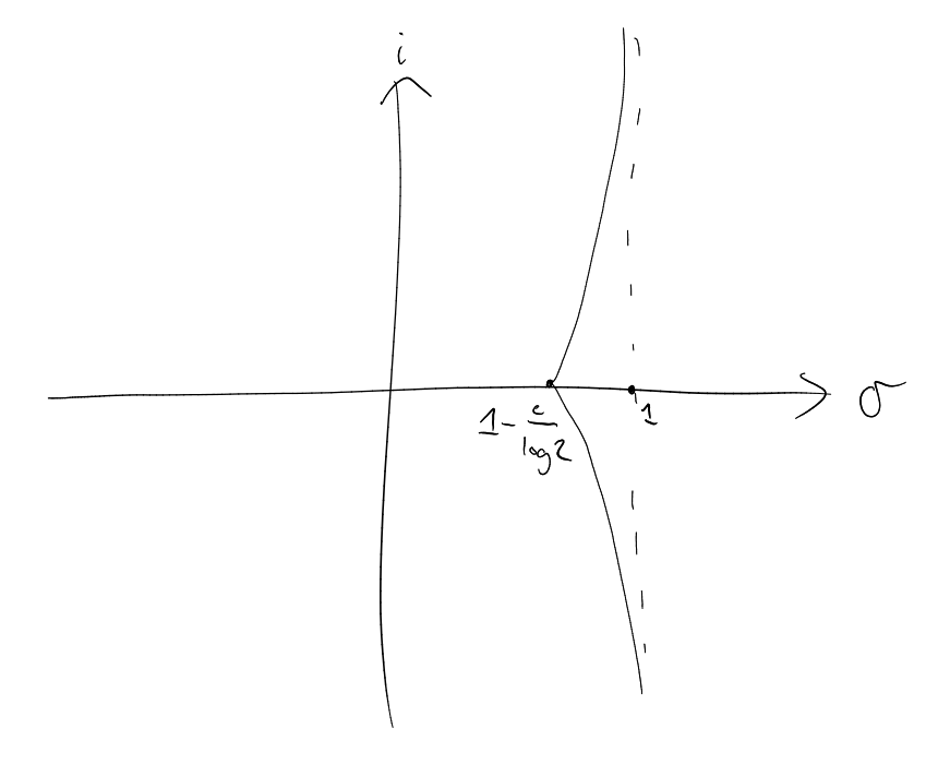
Theorem 3.10 (Zero-free region). There is a constant $c > 0$ such that $ζ (σ + i t) \neq 0$ whenever $σ > 1 - \frac{c}{\log (| t | + 2)}$ . In particular, $ζ (s) \neq 0$ for $Re (s) = 1$ .

Proof. Let $σ \in [1, 2]$ and $t \in ℝ$ . Suppose $ζ (β + i t)$ . uwe know that $β \leq 1$ . We know that $ζ$ has no zeroes in some ball $B (1, r)$ for some $r > 0$ (otherwise the entire function $(s - 1) ζ (s)$ would have an accumulation point for its zeros).

Choosing $c > 0$ small enough, we can assume that $| t | \geq r$ . By the key inequality for $\frac{ζ^{'}}{ζ}$ ,

3 \frac{ζ^{'}}{ζ} (σ) + 4 Re (\frac{ζ^{'}}{ζ} (σ + i t)) . + Re (\frac{ζ^{'}}{ζ} (σ + 2 i t)) . \leq 0 .

Apply partial fraction decomposition of $\frac{ζ^{'}}{ζ}$ . So

\frac{ζ^{'}}{ζ} (s) = - \frac{1}{s - 1} + \sum_{| s - ρ | \leq \frac{1}{10}} \frac{1}{s - ρ} + O (\log (| t | + 2)) . (∗∗)

( $t = Im (s)$ ).

Since $Re (ρ) \leq 1$ for any zero $ρ$ ,

Re \frac{1}{σ + i u - ρ} = \frac{σ - Re (ρ)}{| σ + i u - ρ |^{2}} \geq 0

( $σ > 1$ ).

Discarding terms, we get

- \frac{3}{σ - 1} + \frac{4}{σ - β} \leq C \log (| t | + 2) .

Take $σ = 1 + \frac{s c}{\log (| t | + 2)}$ , and assume $β \geq 1 - \frac{c}{\log (| t | + 2)}$ to get

- 3 \frac{\log (| t | + 2)}{5 c} + 4 \frac{\log (| t | + 2)}{6 c} \leq C (\log | t | + 2) .

Take $c = \frac{1}{16 C}$ to get a contradiction. □

Theorem 3.11 (Bounding $z e t a^{'} ∕ z e t a$ ). Assuming that:

$c > 0$ sufficiently small
$T \geq 0$
$Re (s) \geq - 10$
$| Im (s) | \in [T, T + 1]$
$s$ is at least distance $\frac{c}{\log (T + 2)}$ away from any zero or pole

Then

| \frac{ζ^{'} (s)}{ζ (s)} | ≪_{c} {(\log (T + 2))}^{2} .

Proof. If $s = σ + i t$ with $σ > 10$ , then

\begin{array}{l} | \frac{ζ^{'} (s)}{ζ (s)} | & = | \sum_{n = 1}^{\infty} Λ (n) n^{- s} | \\ \leq \sum_{n = 1}^{\infty} Λ (n) n^{- σ} \\ ≪ 1 \end{array}

Assume then that $Re (s) \in [- 10, 10]$ . Apply ( $* *$ ). Each term satisfies

\begin{array}{l} \frac{1}{| s - ρ |} & \leq \frac{\log (T + 2)}{c} \\ \frac{1}{| s - 1 |} & \leq \frac{\log (T + 2)}{c} \end{array}

We know that there are $O (\log (T + 2))$ zeros with multiplicity having imaginary part $\in [T - 2, T + 2]$ . The claim follows from triangle inequality. □