Spectral Graph Theory - Cambridge III notes

Spectral Graph Theory
Lectured by Victor Souza

1Setting
2Graphs and some of their matrices
2.1Irregular graphs
3Expansion and Cheeger inequality
4Loewner order
4.1One-sided expanders
Index

“linear algebraic methods in combinatorics”

1 Setting

$Ω$ a set (finite), $f : Ω \to ℂ$ , $l^{2} (Ω) : = {f : Ω \to ℂ | \sum_{x} | f (x) |^{2} < \infty}$ .

This generalises subsets: given $S \subseteq Ω$ , can consider $𝟙_{S} : Ω \to ℂ$ (where $x \mapsto 1$ for $x \in S$ , and $x \mapsto 0$ otherwise).

When $S$ contains only a single element, we may use the shorthand $𝟙_{x} = 𝟙_{{x}}$ .

$l^{2} (Ω)$ is a $ℂ$ -vector space, equipped with the inner product $⟨ ∙, ∙ ⟩ : l^{2} (Ω) \times l^{2} (Ω) \to ℂ$ defined by

⟨ f, g ⟩ : = \sum_{x \in Ω} \bar{f (x)} g (x),

and a norm $∥ f ∥_{2}^{2} : = ⟨ f, f ⟩ = \sum_{x} | f (x) |^{2}$ .

Matrix over $Ω$ : $M : Ω \times Ω \to ℂ$ . $M (x, y) = M_{x, y}$ is the $x, y$ entry. $M$ acts on $l^{2} (Ω)$ : for $f \in l^{2} (Ω)$ , $M f \in l^{2} (Ω)$ is given by $(M f) (x) = \sum_{y} M (x, y) f (y)$ . $M (α f + β g) = α M f + β M g$ ( $M$ is a linear map).

Given $M$ , $N$ , can calculate

(M N f) (X) = \sum_{y} \sum_{z} M (x, z) N (z, y) f (y),

so define $(M N) (x, y) = \sum_{z} M (x, z) N (z, y)$ , so that the formula $(M N f) (x) = \sum_{y} (M N) (x, y) f (y)$ holds.

Eigenthings: for $M : Ω \times Ω \to ℂ$ , we say that $λ \in ℂ$ is an eigenvalue with eigenfunction $φ \neq 0$ if $M φ = λ φ$ .

Definition 1.1 (Hermitian). $M$ is Hermitian if $M = M^{H}$ , where $M^{H} (x, y) = \bar{M (y, x)}$ .

If $M$ is Hermitian, then $⟨ M f, g ⟩ = ⟨ f, M g ⟩$ .

Theorem 1.2 (Spectral theorem for Hermitian matrices). Assuming that:

$Ω$ finite
$M : Ω \times Ω \to ℂ$ Hermitian
$| Ω | = n$

Then there exist

λ_{1}, \dots, λ_{n} \in ℝ

and

φ_{1}, \dots, φ) n \in l^{2} (Ω)

non-zero such that

(1)
$M φ_{i} = λ_{i} φ_{i}$
(2)
$⟨ φ_{i}, φ_{j} ⟩ 𝟙_{i = j}$
(3)
$M = \sum_{i = 1}^{n} λ φ_{i} φ_{i}^{H}$
(4)
there exists $U$ orthogonal such that $U M U^{H} = diag (λ_{i})$
(5)
if $M$ is real, then can take $φ$ to be real ( $φ : Ω \to ℝ$ )

Lemma 1.3. Any $M$ has an eigenpair $(λ, φ)$ .

Proof. Want $M f = z f$ for some $z \in ℂ$ . So want $(z I - M) f = 0$ to have a non-trivial solution $f \neq 0$ . This happens if and only if $z I - M$ is singular, which happens if and only if $\det (z I - M) = 0$ .

$z \mapsto \det (z I - M)$ is a degree $n$ polynomial in $ℂ$ (degree $n$ since the leading term is $z^{n}$ ), so the fundamental theorem of algebra shows that there exists $λ \in ℂ$ such that $\det (λ I - M) = 0$ . □

Lemma 1.4. Assuming that:

$M$ is Hermitian

Then all eigenvalues are real

Proof.

\begin{array}{l} \bar{λ} ⟨ φ, φ ⟩ & = ⟨ λ φ, φ ⟩ \\ = ⟨ M φ, φ ⟩ \\ = ⟨ φ, M φ ⟩ \\ = ⟨ φ, λ φ ⟩ \\ = λ ⟨ φ, φ ⟩ \end{array}

Since $φ \neq 0$ , $⟨ φ, φ ⟩ = ∥ φ ∥^{2} > 0$ , hence $λ = \bar{λ}$ , i.e. $λ \in ℝ$ . □

Lemma 1.5. Assuming that:

$M$ Hermitian
$λ_{i} \neq λ_{j}$ are eigenvalues of $M$ with eigenvectors $φ_{i}$ , $φ_{j}$

Then

⟨ φ_{i}, φ_{j} ⟩ = 0

Proof.

\begin{array}{l} λ_{i} ⟨ φ_{i}, φ_{j} ⟩ & = ⟨ M φ_{i}, φ_{j} ⟩ \\ = ⟨ φ_{i}, M φ_{j} ⟩ \\ = λ_{j} ⟨ φ_{i}, φ_{j} ⟩ \end{array}

Since we assumed $λ_{i} \neq λ_{j}$ , this gives $⟨ φ_{i}, φ_{j} ⟩ = 0$ . □

Lemma 1.6. Assuming: - $M$ is real symmetric - $λ$ is an eigenvalue Then: there exists $g : Ω \to ℝ$ such that $M g = λ g$ .

Proof. Let $φ = f + i g$ . Then $M φ = M f + i M g = λ φ = λ f + i λ g$ . Hence $M f = M λ$ and $M g = λ g$ . So either $f$ or $g$ works. □

Notation. For $f, g \in l^{2} (Ω)$ , $f g^{H}$ denotes the matrix $(f g^{H}) (x, y) = f (x) \bar{g} (y)$ .

“ $(f g^{H}) h = f g^{H} h = f ⟨ g, h ⟩$ ”

Proof of Spectral theorem for Hermitian matrices. Using the above lemmas, can find $λ_{n} \in ℝ$ and $φ_{i} : Ω \to ℂ$ non-zero such that $M φ_{n} = λ_{n} φ_{n}$ and $∥ φ_{n} ∥ = 1$ .

Then let $M^{'} = M - λ_{n} φ_{n} φ_{n}^{H}$ . $l^{2} (Ω) = span (φ_{n}) \oplus span {(φ_{n})}^{⊤}$ . Then check that $M^{'}$ acts on $span {(φ_{n})}^{⊤}$ and use induction. □

Theorem 1.7 (Courant-Fischer-Weyl Theorem). Assuming: - $M : Ω \times Ω \to ℝ$ symmetric - eigenvalues $λ_{1} \leq \dots \leq λ_{n}$ Then:

λ_{k} = \min_{\begin{array}{c} W \leq l^{2} (Ω) \\ \dim W = k \end{array}} \max_{\begin{array}{c} f \in W \\ f \neq 0 \end{array}} \frac{⟨ f, M f ⟩}{⟨ f, f ⟩} = F_{k} .

Definition 1.8 (Rayleigh quotient). $\frac{⟨ f, M f ⟩}{⟨ f, f ⟩}$ is called the Rayleigh quotient.

Proof. Let $W^{'} = span (φ_{1}, \dots, φ_{k})$ . Note

F_{k} \leq \max_{\begin{array}{c} f \in W \\ f \neq 0 \end{array}} \frac{⟨ f, M f ⟩}{⟨ f, f ⟩} .

For $f \in W$ , $f = \sum_{i = 1}^{k} α_{i} φ_{i}$ , so

\frac{⟨ f, M f ⟩}{⟨ f, f ⟩} = \frac{\sum_{i = 1}^{k} α_{i}^{2} λ_{i}}{\sum_{i = 1}^{k} α_{i}^{2}} \leq \frac{λ_{k} \sum_{i = 1}^{k} α_{i}^{2}}{\sum_{i = 1}^{k} α_{i}^{2}} = λ_{k} .

So $F_{k} \leq λ_{k}$ .

Now suppose $W$ is a subspace with $\dim W = k$ . Let $V = span (φ_{k}, \dots, φ_{n})$ , and note $\div V = n - k + 1$ . Note

\dim (V \cap W) = \dim V + \dim W - \dim (V + W) \geq k + (n - k + 1) - n = 1 .

So for all such $W$ , there exists $f \in V \cap W$ , $f \neq 0$ such that $f = \sum_{i \geq k} α_{i} φ_{i}$ . Then

⟨ f, M f ⟩ = \sum_{i \geq k} α_{i}^{2} λ_{i} \geq λ_{k} \sum_{i \geq k} α_{i}^{2} = λ_{k} ⟨ f, f ⟩,

so $F_{k} \geq λ_{k}$ . □

Notation 1.9. Define $Q_{M} : l^{2} (Ω) \to ℂ$ by $Q_{M} (f) = ⟨ f, M f ⟩ = \sum_{x, y} f (x) M (x, y) f (y)$ .

Define $q_{m} (f) = \frac{Q_{M} (f)}{Q_{I} (f)}$ .

$λ_{1} (M) = \min_{f \neq 0} q_{M} (f)$ and it is attained only on

Lemma 1.10. eigenfunctions of $λ_{1}$ .

Proof. Let $f = \sum_{i} α_{i} φ_{i}$ and $M f = \sum_{i} α_{i} λ_{i} φ_{i}$ . Then

\begin{array}{l} Q_{M} (f) & = ⟨ f, M f ⟩ \\ \sum_{i, j} α_{i} α_{j} λ_{i} ⟨ φ_{i}, φ_{j} ⟩ \\ = \sum_{i} α_{i}^{2} λ_{i} \end{array}

and

q_{M} (f) = \frac{\sum_{i} α_{i}^{2} λ_{i}}{\sum_{i} α_{i}^{2}} \geq λ_{i} .

Equality occurs here if and only if $\sum_{i} (λ_{1} - λ_{i}) α_{i}^{2} = 0$ . So $α_{i} = 0$ whenever $λ_{i} > λ_{1}$ . □

Assuming:

Lemma 1.11. - $φ_{1}$ is an eigenfunction of $λ_{1}$ . Then: $λ_{2} (M) = \min_{\begin{array}{c} f ⊥ φ_{1} \\ f \neq 0 \end{array}} q_{M} (f)$ , and it is attained only on eigenfunctions of $λ_{2} (M)$ .

Proof.

q_{M} (f) = \frac{\sum_{i} α_{i}^{2} λ_{i}}{\sum_{i} α_{i}^{2}} \geq \frac{α_{1}^{2} λ_{1} + (\sum_{i \geq 2} α_{i}^{2}) λ_{2}}{\sum_{i} α_{i}^{2}} .

\min_{\begin{array}{c} f ⊥ φ_{i} \\ f \neq 0 \end{array}} q_{M} (f) \geq λ_{2} .

Deal with the equality case similarly to before. □

In general:

λ_{k} (M) = \min_{\begin{array}{c} f ⊥ φ_{1}, \dots, φ_{k - 1} \\ f \neq 0 \end{array}} q_{M} (f) .

(and equality case is similar to before). Also,

\begin{array}{l} λ_{n} (M) & = \max_{f \neq 0} q_{M} (f) \\ λ_{n - k} (M) & = \max_{\begin{array}{c} f ⊥ φ_{n}, \dots, φ_{n - k + 1} \\ f \neq 0 \end{array}} q_{M} (f) \end{array}

(and equality case is similar to before).

2 Graphs and some of their matrices

Graph $G = (V, E)$ : set of vertices $V$ , $| V | = n$ , $E$ is a set of (unordered) pairs of vertices.

Definition 2.1 (Adjacency matrix). The adjacency matrix of a graph $G$ is the matrix $A_{G} : V \times V \to ℝ$ defined by

A_{G} (x, y) = {\begin{matrix} 1 & {x, y} \in E (G) \\ 0 & {x, y} \notin E (G) \end{matrix}

Definition 2.2 (Degree matrix). The degree matrix of a graph $G$ is the matrix $D_{G} : V \times V \to ℝ$ defined by

D_{G} (x, y) = {\begin{matrix} \deg (x) & x = y \\ 0 & otherwise \end{matrix}

Definition 2.3 (Laplacian matrix). The Laplacian matrix of a graph $G$ is defined by $L_{G} = D - A$ .

We can now calculate:

\begin{array}{l} Q_{A} (f) & = \sum_{x, y} f (x) A (x, y) f (y) \\ = 2 \sum_{x \sim y} f (x) f (y) \\ Q_{D} (f) & = \sum_{x, y} f (x) D (x, y) f (y) \\ = \sum_{x} f {(x)}^{2} \deg (x) \\ = \sum_{x} f {(x)}^{2} \sum_{y} A (x, y) \\ = \sum_{x, y} f {(x)}^{2} A (x, y) \\ = \frac{1}{2} \sum_{x, y} (f {(x)}^{2} + f {(y)}^{2}) A (x, y) \\ = \sum_{x \sim y} (f {(x)}^{2} + f {(y)}^{2}) \\ Q_{L} (f) & = Q_{D - A} (f) \\ = Q_{D} (f) - Q_{A} (f) \\ = \sum_{x \sim y} (f {(x)}^{2} + f {(y)}^{2} - 2 f (x) f (y)) \\ = \sum_{x \sim y} {(f (x) - f (y))}^{2} \\ \geq 0 \end{array}

Corollary 2.4. For any graph $G$ , $L_{G}$ is a positive semi definite matrix with eigenvector $1$ , which has eigenvalue $1$ .

Proof. Since $Q_{L} (f) = \sum_{x \sim y} {(f (x) - f (y))}^{2}$ , we see that $Q_{L} (f) \geq 0$ , with equality when $f$ is constant. □

Proposition 2.5. $λ_{2} (L_{g}) > 0$ if and only if $G$ is connected. $λ_{k} (L_{G}) = 0$ if and only if $G$ has at least $k$ connected components.

Proof.

λ_{2} = \min_{\begin{array}{c} f ⊥ 1 \\ f \neq 0 \end{array}} \frac{\sum_{x \sim y} {(f (x) - f (y))}^{2}}{⟨ f, f ⟩} \geq 0

Equality happens if and only if $Q_{L} (f) = 0$ , which happens if and only if $f$ is constant on connected components. The dimension of ${f : constant on connected components}$ is the number of connected components of $G$ .

TODO? □

TODO

2.1 Irregular graphs

$A$ , $D$ , $L = D - A$ , $Q_{L} (f) = \sum_{x \sim y} {(f (x) - f (y))}^{2}$ , $q_{L} (f) = \frac{\sum_{x \sim y} {(f (x) - f (y))}^{2}}{\sum_{x} f {(x)}^{2}}$ .

\begin{array}{l} Q_{L} (f) & = ⟨ f, L f ⟩ \\ = ⟨, (D - A) f ⟩ \\ = ⟨ f, (2 D - (D + A)) f ⟩ \\ = ⟨ f, 2 D f ⟩ - ⟨ f, (D + A) f ⟩ \end{array}

When $G$ is $d$ -regular,

{\tilde{L}}_{G} = \frac{1}{d} L_{G} = I - \frac{1}{d} A_{G},

$λ_{i} ({\tilde{L}}_{G} \in [0, 2]$ .

q_{\tilde{L}} (f) = \frac{\sum_{x \sim y} {(f (x) - f (y))}^{2}}{\sum_{x} d (x) f {(x)}^{2}} = 2 - \frac{\sum_{x \sim y} {(f (x) + f (y))}^{2}}{\sum_{x} d (x) f {(x)}^{2}} .

Want $M$ such that $q_{M} (f)$ equals the expression above. Recall $q_{M} (f) = \frac{⟨ f, M f ⟩}{⟨ f, f ⟩}$ . But the above expression is $\frac{⟨ f, M f ⟩}{⟨ f, D f ⟩}$ .

Let $D^{\frac{1}{2}} (x, y) = 𝟙_{x = y} \sqrt{d (x)}$ . Assume $d (x) \geq 1$ for all $x \in G$ . Note

q_{M} (D^{\frac{1}{2}} f) = \frac{⟨ D^{\frac{1}{2}} f, M D^{\frac{1}{2}} f ⟩}{⟨ D^{\frac{1}{2}} f, D^{\frac{1}{2}} f ⟩} = \frac{⟨ f, D^{\frac{1}{2}} M D^{\frac{1}{2}} f ⟩}{⟨ f, D f ⟩} .

Want $D^{\frac{1}{2}} M D^{\frac{1}{2}} = L = D - A$ . Define

{\tilde{L}}_{G} = D^{- \frac{1}{2}} (D - A) D^{- \frac{1}{2}} = I - D^{- \frac{1}{2}} A D^{- \frac{1}{2}} .

{\tilde{L}}_{G} = {\begin{matrix} 1 & if x = y \\ - \frac{1}{\sqrt{d (x) d (y)}} & if x \neq y and x \sim y \\ 0 & if x \neq y and x ⁄ \sim y \end{matrix}

Also,

q_{{\tilde{L}}_{G}} (D^{\frac{1}{2}} f) = \frac{\sum_{x \sim y} {(f (x) - y (y))}^{2}}{\sum_{x} d (x) f {(x)}^{2}} .

We have

λ_{k} ({\tilde{L}}_{G}) = \min_{\dim W = K} \max_{\begin{array}{c} f \in W \\ f \neq 0 \end{array}} q_{{\tilde{L}}_{G}} (D^{\frac{1}{2}} f) .

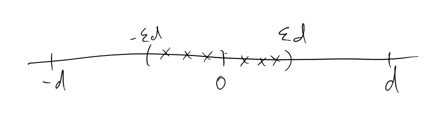
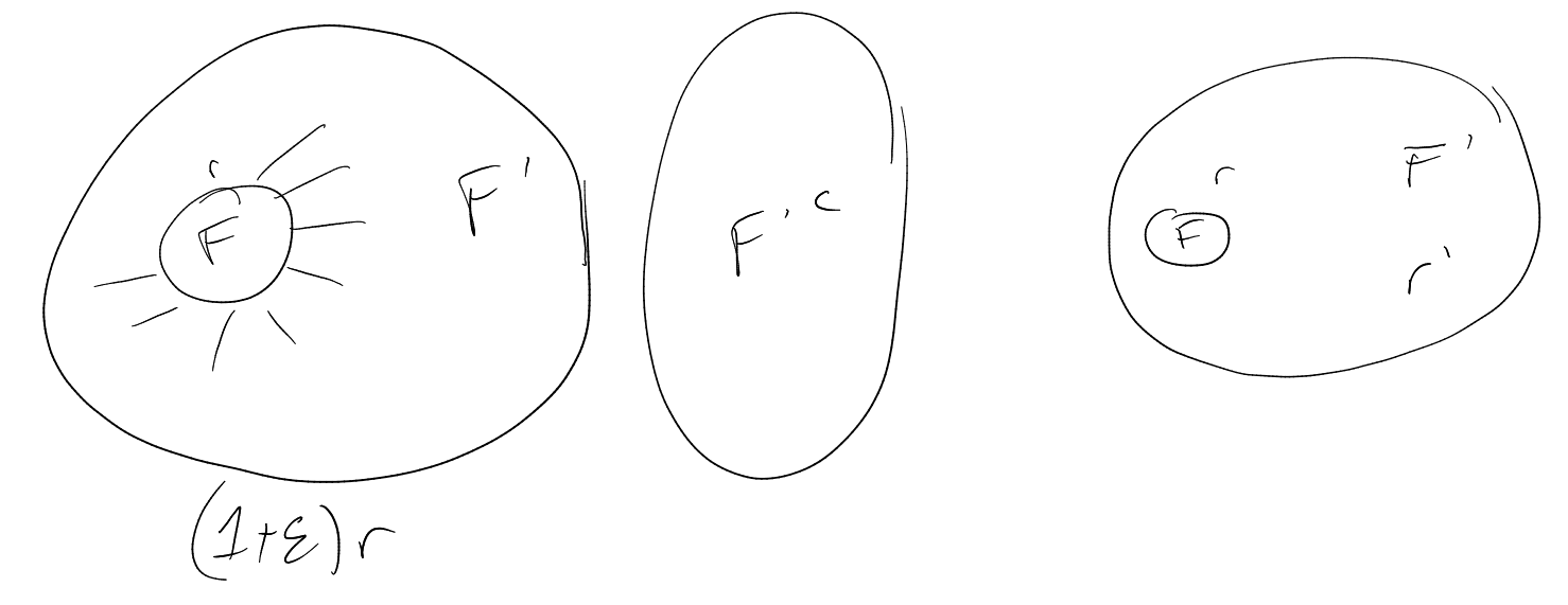
3 Expansion and Cheeger inequality

Assume $G$ is $d$ -regular. Write $G = (V, E)$ .

Definition 3.1 (Expansion). Given a $d$ -regular graph $G$ and $S \subseteq V$ , the expansion of $S$ is

Φ (S) : = \frac{e (S, V ∖ S)}{d | S |} .

Note that $0 \leq Φ \leq 1$ , for example because

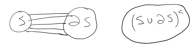
Φ (S) = ℙ_{\begin{array}{c} x \sim U (S) \\ y \sim N (x) \end{array}} (y \notin S) .

Definition 3.2 (Edge expansion). The (edge) expansion of a cut $(S, V ∖ S)$ is defined as

Φ (S, V ∖ S) : = \max {Φ (S), Φ (V ∖ S)} = \frac{e (S, V ∖ S)}{d \min {| S |, | V ∖ |}} .

Definition 3.3 (Edge expansion of a graph). The edge expansion of a graph is

Φ (G) : = \min_{\begin{array}{c} S \subseteq V \\ \emptyset \neq S \neq V \end{array}} Φ (S, V ∖ S) = \min_{\begin{array}{c} S \subseteq V \\ 0 < | S | < | V | ∕ 2 \end{array}} Φ (S) .

Theorem 3.4 (Cheeger’s inequality). Assuming that:

$G$ be $d$ -regular

Then

\frac{λ_{2} ({\tilde{L}}_{G})}{2} \leq Φ (G) \leq \sqrt{2 λ_{2} ({\tilde{L}}_{G})} .

Consider $𝟙_{S} : V \to ℝ$ , where $𝟙_{S} (x) = 1$ if $x \in S$ and $𝟙_{S} (x) = 0$ otherwise. Then

\begin{array}{l} Q_{L} (𝟙_{S}) & = \sum_{x \sim y} {(𝟙_{S} (x) - 𝟙_{S} (y))}^{2} = e (S, V ∖ S) \\ q_{\tilde{L}} (𝟙_{S}) & = \frac{e (S, V ∖ S)}{d | S |} = Φ (S) \end{array}

Recall

λ_{2} ({\tilde{L}}_{G}) = \min_{\dim W = 2} \max_{\begin{array}{c} f \in W \\ f \neq 0 \end{array}} q_{{\tilde{L}}_{G}} (f) .

We pick $W = span {𝟙_{S}, 𝟙_{V ∖ S}}$ . Note

\begin{array}{l} λ_{2} ({\tilde{L}}_{G}) & \leq \max_{\begin{array}{c} α, β \\ (α, β) \neq (0, 0) \end{array}} q_{{\tilde{L}}_{G}} (α 𝟙_{S} + β 𝟙_{V ∖ S}) \\ \leq \max_{α, β} 2 \max {q_{\tilde{L} (G)} (α 𝟙_{S}), q_{{\tilde{L}}_{G}} (β 𝟙_{V ∖ S})} \end{array}

Lemma 3.5. Assuming that:

$M$ is symmetric positive semi-definite
$⟨ f, g ⟩ = 0$

Then

q_{M} (f + g) \leq 2 \max {q_{M} (f), q_{M} (g)} .

Proof. Let $λ_{i}$ , $φ_{i}$ such that $f = \sum_{i} λ_{i} φ_{i}$ and $g = \sum_{i} β_{i} φ_{i}$ . Then

q_{M} (f + g) = \frac{\sum_{i} λ_{i} {(α_{i} + β_{i})}^{2}}{∥ f + g ∥^{2}} \leq \frac{\sum_{i} λ_{i} (2 α_{i}^{2} + 2 β_{i}^{2})}{∥ f ∥^{2} + ∥ g ∥^{2}} .

Then

\begin{array}{l} q_{M} (f + g) & \leq 2 (\frac{\sum_{i} λ_{i} α_{i}^{2} + \sum_{i} λ_{i} β_{i}^{2}}{∥ f ∥^{2} + ∥ g ∥^{2}}) \\ = 2 (\frac{q_{M} (f) ∥ f ∥^{2} + q_{M} (g) ∥ g ∥^{2}}{∥ f ∥^{2} + ∥ g ∥^{2}}) \\ \leq 2 \max {q_{M} (f), q_{M} (g)} □ \end{array}

Proof of left inequality in Cheeger’s inequality. $λ_{2} \leq 2 \max {Φ (S), Φ (V ∖ S)} = 2 Φ (S, V ∖ S)$ . Then minimise over all $S$ , to get $λ_{2} \leq 2 Φ (G)$ . □

Recall that

Φ (S) = q_{{\tilde{L}}_{G}} (𝟙_{S})

and

Φ (G) = \min_{\begin{array}{c} S \subseteq V \\ 1 \leq | S | \leq | V | ∕ 2 \end{array}} q_{{\tilde{L}}_{G}} (𝟙_{S}) .

Fiedler’s Algorithm

Input: $G, φ : V \to ℝ$ .

Sort vertices $x_{1}, \dots, x_{n}$ such that $φ (x_{1}) \leq \dots \leq φ (x_{n})$ .
Find cut $K$ that minimises $Φ ({x_{2}, \dots, x_{k}}, {x_{k + 1}, \dots, x_{n}})$ .

Output: The cut.

Running time: $O (| V | \log | V | + | E |)$ .

Lemma 3.6. Assuming that:

$ψ : V \to ℝ$
$⟨ ψ, 1 ⟩ = 0$
let $(S, V ∖ S) = Fiedler (G, ψ)$

Then

Φ (S, V ∖ S) \leq \sqrt{2 q_{{\tilde{L}}_{G}} (ψ)} .

If $ψ : V \to ℝ$ , call a cut $({x : ψ (x) \geq τ)}, {x : ψ (x) < τ})$ a threshold cut for $ψ$ .

Lemma 3.7. Assuming that:

$φ : V \to ℝ$
$⟨ φ, 1 ⟩ = 0$

Then there is

ψ : V \to ℝ_{\geq 0}

such that

q_{{\tilde{L}}_{G}} (ψ) \leq q_{{\tilde{L}}_{G}} (ψ)

| supp ψ | = | {x : ψ (x) > 0} | \leq \frac{| V |}{Q}

and any threshold cut for

ψ

is a threshold cut for

φ

Lemma 3.8. Assuming that:

$ψ : V \to ℝ_{\geq 0}$

Then there is

0 < t \leq ∥ ψ ∥_{\infty}

such that

Φ ({x : ψ (x) \geq t}) \leq \sqrt{2 q_{{\tilde{L}}_{G}} (ψ)} .

Proof of Lemma 3.7. If $⟨ φ, 1 ⟩ = 0$ then

\begin{array}{l} q_{{\tilde{L}}_{G}} (φ + α 1) & = \frac{Q_{{\tilde{L}}_{G}} (φ + α 1)}{∥ φ + α 1 ∥^{2}} \\ = \frac{Q_{{\tilde{L}}_{G}} (φ)}{∥ φ ∥^{2} + α^{2}} \\ \leq \frac{Q_{{\tilde{L}}_{G}} (φ)}{∥ φ ∥^{2}} \\ = q_{{\tilde{L}}_{G}} (φ) \end{array}

Let $m \in ℝ$ be the median of $φ$ .

\begin{array}{l} | {x \in V : φ (x) > m} | & \leq \frac{| V |}{2} \\ | {x \in V : φ (x) < m} | & \leq \frac{| V |}{2} \end{array}

$\bar{φ} = φ - m 1$ , $q_{{\tilde{L}}_{G}} (\bar{φ}) \leq q_{{\tilde{L}}_{G}} (φ)$ . Let $\bar{φ} = {\bar{φ}}^{+} - {\bar{φ}}^{-}$ , where ${\bar{φ}}^{+}, {\bar{φ}}^{-} : V \to ℝ_{\geq 0}$ . So

\bar{φ} (x) = {\begin{matrix} {\bar{φ}}^{+} (x) & φ (x) > m \\ - {\bar{φ}}^{-} (x) & φ (x) < m \\ 0 & φ (x) = m \end{matrix} .

Note $⟨ {\bar{φ}}^{-}, {\bar{φ}}^{+} ⟩ = 0$ .

Claim: either ${\bar{φ}}^{+}$ or ${\bar{φ}}^{-}$ suffices.

\begin{array}{l} q_{{\tilde{L}}_{G}} (φ) & \geq q_{{\tilde{L}}_{G}} (\bar{φ}) \\ = q_{{\tilde{L}}_{G}} ({\bar{φ}}^{+} - {\bar{φ}}^{-}) \\ = \frac{\sum_{x \sim y} {({\bar{φ}}^{+} (x) - {\bar{φ}}^{-} (x) - {\bar{φ}}^{+} (y) + {\bar{φ}}^{-} (y))}^{2}}{∥ {\bar{φ}}^{+} - {\bar{φ}}^{-} ∥^{2}} \\ = \frac{\sum_{x \sim y} (({\bar{φ}}^{+} (x) - {\bar{φ}}^{+} (y)) - {({\bar{φ}}^{-} (x) - {\bar{φ}}^{-} (x))}^{2}}{∥ {\bar{φ}}^{+} ∥^{2} + ∥ {\bar{φ}}^{-} ∥^{2}} \\ \geq \frac{\sum_{x \sim y} {({\bar{φ}}^{+} (x) - {\bar{φ}}^{+} (y))}^{2} + {({\bar{φ}}^{-} (x) - {\bar{φ}}^{-} (y))}^{2}}{∥ {\bar{φ}}^{+} ∥^{2} + ∥ {\bar{φ}}^{-} ∥^{2}} \\ = \frac{q_{{\tilde{L}}_{G}} ({\bar{φ}}^{+}) ∥ \bar{φ} ∥^{2} + q_{{\tilde{L}}_{G}} ({\bar{φ}}^{-}) ∥ {\bar{φ}}^{-} ∥^{2}}{∥ \bar{φ} ∥^{2} + ∥ {\bar{φ}}^{-} ∥^{2}} \end{array}

□

Proof of Lemma 3.8. Assume $∥ ψ ∥_{\infty} = 1$ . We find $0 < t \leq 1$ . Choose $t$ at random, such that $t^{2} \sim Unif ([0, 1])$ . Let

S_{t} = {x \in V : ψ (x) > t} .

Then

𝔼 | S_{t} | = \sum_{x} ℙ (x \in S_{t}) = \sum_{x} ℙ (ψ {(x)}^{2} > t^{2}) = \sum_{x} ψ {(x)}^{2} .

Have

Φ (S_{t}) = \frac{e (S_{t}, V ∖ S_{t})}{d | S_{t} |} .

Also, can calculate:

\begin{array}{l} 𝔼 d | S_{t} | & = d \sum_{x} ψ {(x)}^{2} \\ 𝔼 e (S_{t}, V ∖ S_{t}) & = \sum_{x \sim y} ℙ (x y is cut by (S_{t}, V ∖ S_{t})) \\ = \sum_{x \sim y} | ψ {(x)}^{2} - ψ {(y)}^{2} | \\ = \sum_{x \sim y} | ψ (x) - ψ (y) | (ψ (x) + ψ (y)) \\ \leq \sqrt{\sum_{x \sim y} {(ψ (x) - ψ (y))}^{2}} \cdot \sqrt{\sum_{x \sim y} {(ψ (x) + ψ (y))}^{2}} \end{array}

Then

\begin{array}{l} \frac{𝔼 e (S_{t}, V ∖ S_{t})}{𝔼 d | S_{t} |} & \leq \sqrt{q_{{\tilde{L}}_{G}} (ψ)} \cdot \sqrt{\frac{\sum_{x \sim y} {(ψ (x) + ψ (y))}^{2}}{d \sum_{x} ψ {(x)}^{2}}} \\ \leq \sqrt{2 q_{{\tilde{L}}_{G}} (ψ)} \end{array}

Now use the following fact to finish:

Fact: If $X$ and $Y$ are random variables with $ℙ (Y > 0) = 1$ , then $ℙ (\frac{X}{Y} \leq \frac{𝔼 X}{𝔼 Y})$ .

(Proof: let $R = \frac{𝔼 X}{𝔼 Y}$ . Then $𝔼 (X - R Y) = 0$ , so $ℙ (X - R Y \leq 0)) > 0$ , hence $ℙ (\frac{X}{Y} \leq R) > 0$ ). □

Example. $C_{N}$ . This has $λ_{2} ({\tilde{L}}_{C_{N}} = 𝜃 (\frac{1}{N^{2}})$ .

For $S \subseteq C_{N}$ with $| 1 \leq S | \leq \frac{1}{2} | C_{N} |$ , we have $e (S, V ∖ S) \geq 2$ . So

Φ (S) = \min_{\begin{array}{c} S \subseteq V \\ 0 < | S | < | V | ∕ 2 \end{array}} \frac{e (S, V ∖ S)}{d | S |} = \min_{1 \leq s \leq N ∕ 2} \frac{2}{2 s} ≃ \frac{2}{N} .

Compare with Cheeger’s inequality:

\frac{1}{N^{2}} < \frac{1}{N} \leq \sqrt{\frac{1}{N^{2}}} .

Example. $G = Q_{n}$ , $N = 2^{n}$ . $G = Cay ({(ℤ ∕ 2 ℤ)}^{n}, {e_{1}, \dots, e_{n}})$ . We index eigenfunctions by sets $T \subseteq [n]$ . $χ_{T} (x) = {(- 1)}^{\sum_{i \in T} x_{i}}$ , $λ_{T} = \frac{2 | T |}{n}$ .

$λ_{2}^{(} {\tilde{L}}_{Q_{n}}) = \frac{2}{n} = \frac{2}{\log N}$ .

$Φ (Q_{n}) \geq \frac{2}{2 n} = \frac{1}{n}$ . If $S \subseteq Q_{n}$ , $| S | \leq N ∕ 2$ , then

\frac{e (S, V ∖ S)}{n | S |} \geq \frac{1}{n} ⟹ e (S, V ∖ S) \geq | S | .

Harper gives a better bound:

e (S, V ∖ S) \geq | S | \log_{2} (\frac{2^{n}}{| S |}) .

By considering $S$ being half of the cube, we get

Φ (Q_{n}) = \frac{1}{n} = \frac{λ_{2} ({\tilde{K}}_{Q_{n}})}{2} .

Fiedler’s algorithm: Let $f = \sum_{i = 1}^{n} χ_{{i}}$ , ${\tilde{L}}_{Q_{n}} f = \frac{2}{n} f$ . $f (x) = \sum_{i = 1}^{n} {(- 1)}^{x_{i}} = n - 2 | x |$ .

Φ_{k} = \frac{(\binom{n}{k}) (n - k)}{n \sum_{j = 0}^{k} (\binom{n}{j})} .

$k = \frac{n}{2}$ ,

\frac{(\binom{n}{n ∕ 2}) \frac{n}{2}}{n 2^{n - 1}} = \frac{(\binom{n}{n ∕ 2})}{2^{n}} \approx \frac{1}{\sqrt{n}} .

4 Loewner order

Definition 4.1 (Loewner order). For $A$ , $B$ matrices, write $A ≼ B$ if $B - A$ is positive semidefinite. In particular, $A ≽ 0$ if and only if $A$ is positive semidefinite.

$q_{A} (f) = \frac{⟨ f, A f ⟩}{⟨ f, f ⟩} = 0$ .

$A ≼ B$ if and only if $\forall f \neq 0$ ,

\frac{⟨ f, A f ⟩}{⟨ f, f ⟩} \leq \frac{⟨ f, B f ⟩}{⟨ f, f ⟩} .

$⟨ f, A f ⟩ \leq ⟨ f, B f ⟩$ .

This is indeed an order: $A ≼ B ≼ C$ implies $A ≼ C$

⟨ f, A f ⟩ \leq ⟨ f, B f ⟩ \leq ⟨ f, C f ⟩ .

If $A ≼ B$ , then $λ_{k} (A) \leq λ_{k} (B)$ .

λ_{k} (A) = \min_{\dim W = k} \max_{\begin{array}{c} f \in W \\ f \neq 0 \end{array}} \frac{⟨ f, A f ⟩}{⟨ f, f ⟩} .

$A ≼ B$ if and only if $A + C ≼ B + C$ .

If $G$ is a graph, then $L_{G} ≼ 0$ .

Definition 4.2 (eps-approximation). $G$ is an $𝜀$ -approximation of $H$ if

(1 - 𝜀) L_{H} ≼ L_{G} ≼ (1 + 𝜀) L_{H} .

Lemma 4.3. Given the definition $∥ M ∥ = \max_{f \neq 0} \frac{∥ M f ∥}{∥ f ∥}$ (for $M$ symmetric), we have $∥ M ∥ = \max {| λ_{k} (M) |}$ .

Proof. $f = \sum_{i} α_{i} φ_{i}$ , $M φ_{i} = λ_{i} φ_{i}$ , $∥ f ∥^{2} = \sum_{i} α_{i}^{2}$ ,

∥ M f ∥^{2} = {∥ \sum_{i} α_{i} λ_{i} φ_{i} ∥}^{2} = \sum_{i} α_{i}^{2} λ_{i}^{2} .

\frac{∥ M f ∥}{∥ f ∥} = \sqrt{\frac{\sum_{i} α_{i}^{2} λ_{i}^{2}}{\sum_{i} α_{i}^{2}}} \leq \max_{k} | λ_{k} | . □

Lemma 4.4. Assuming: - $G$ is an $𝜀$ -approximation of $H$ Then: $∥ L_{G} - L_{H} ∥ \leq 𝜀$ .

Proof. $- 𝜀 {\tilde{L}}_{H} ≼ {\tilde{L}}_{G} - {\tilde{L}}_{H} ≼ 𝜀 {\tilde{L}}_{H}$ . $λ_{k} ({\tilde{L}}_{G} - {\tilde{L}}_{H}) \leq λ_{k} ({\tilde{L}}_{H}) \leq 2 𝜀$ . □

Definition ((d,eps)-expander). $G = (V, E)$ , $| V | = n$ is a $(d, 𝜀)$ -expander if $G$ is an $𝜀$ -approximation of $\frac{d}{n} K_{n}$ .

Equivalent:

(1 - 𝜀) \frac{d}{n} L_{K_{n}} ≼ L_{G} ≼ (1 + 𝜀) \frac{d}{n} L_{K_{n}} .

$L_{K_{n}} = (n - 1) I - A_{K_{n}} = n I - J$ , where $J$ is the all ones matrix ( $J (x, y) = 1$ ). If $f ⊥ q$ , then $J f = ⟨ f, 1 ⟩ f = 0$ . In this case, $L_{K_{n}} f = n I f - J f = n f$ .

So $λ_{k} (L_{K_{n}}) = n$ for $k \geq 0$ .

(1 - 𝜀) \frac{d}{n} (n I - J) ≼ d I - A_{G} ≼ (1 + 𝜀) \frac{d}{n} (n I - J)

- 𝜀 \frac{2}{n} (n I - J) ≼ d I - A_{G} - \frac{d}{n} (n I - J) ≼ 𝜀 \frac{d}{n} (n I - J)

- 𝜀 (d I - \frac{d}{n} J) ≼ \frac{d}{n} J - A_{G} ≼ 𝜀 (d I - \frac{d}{n} J)

For $f ⊥ 1$ , $- 𝜀 d ⟨ f, f ⟩ \leq - ⟨ f, A f ⟩ \leq 𝜀 d ⟨ f, f ⟩$ .

So $G$ is a $(d, 𝜀)$ -expander if and only if

| λ_{k} (A_{G}) | \leq 𝜀 d

for all $1 \leq k \leq n - 1$ .

Lemma 4.5 (Expander Mixing Lemma). Assuming that:

$G$ is $d$ -regular
$G$ is a $(d, 𝜀)$ -expander

Then

\forall S, T \subseteq V

| e (S, T) - \frac{d}{n} | S | | T | | \leq \frac{𝜀 d}{n} \sqrt{| S | | T | | S^{c} | | T^{c} |} .

Proposition 4.6. Assuming that:

$G$ a $d$ -regular graph on $n$ vertices
$λ, 𝜀 > 0$ , $𝜀 d = λ$

Then the following are equivalent:

(i) $G$ is a $(n, d, λ)$ -graph
(ii) $λ_{k} (A_{G}) ∋ [- λ, λ]$ , for $1 \leq k \leq n - 1$
(iii) $λ_{k} (L_{G}) \in [d - λ, d + λ]$ for $2 \leq k \leq n$
(iv) $λ_{k} ({\tilde{L}}_{G}) \in [1 - \frac{λ}{d}, 1 + \frac{λ}{d}] = [1 - 𝜀, 1 + 𝜀]$ for $1 \leq k \leq n$
(v) $(1 - 𝜀) \frac{d}{n} L_{K_{n}} ≼ L_{G} ≼ (1 + 𝜀) \frac{d}{n} L_{K_{n}}$
(vi) $G$ is $(d, 𝜀)$ -expander (also $(d, \frac{λ}{d})$ -expander)
(vii) $∥ L_{G} - \frac{d}{n} L_{K_{n}} ∥ \leq 𝜀 d = λ$
(viii) $∥ A_{G} - \frac{d}{n} J ∥ \leq 𝜀 d = λ$

Lemma 4.7 (Expander Mixing Lemma). Assuming that:

$G = (V, E)$ an $(n, d, λ)$ -graph
$S, T \subseteq V$ (and define $e (S, T) = \sum_{x \in S} \sum_{y \in T} 𝟙_{x y \in E}$ )

Then

\begin{array}{l} | e (S, T) - \frac{d}{n} | S | | T | | & \leq \frac{λ}{n} \sqrt{| S | | S^{c} | | T | | T^{c} |} \\ \leq λ \sqrt{| S | | T |} \end{array}

Proof. $⟨ 𝟙_{S}, L_{G} 𝟙_{T} ⟩ = ⟨ 𝟙_{S}, (d I - A_{G}) 𝟙_{T} ⟩$ , $⟨ 𝟙_{S}, d I 𝟙_{T} ⟩ = d | S \cap T |$ .

\begin{array}{l} ⟨ 𝟙_{S}, A_{G} 𝟙_{T} ⟩ & = \sum_{x} \sum_{y} 𝟙_{S} (x) A_{G} (x, y) 𝟙_{T} (y) \\ = \sum_{x} \sum_{y} 𝟙_{x y \in E} \\ = e (S, T) \end{array}

$\frac{d}{n} L_{K_{n}} = d I - \frac{d}{n} J$ .

⟨ 𝟙_{S}, \frac{d}{n} J 𝟙_{T} ⟩ = \frac{d}{n} ⟨ 𝟙_{S}, J 𝟙_{T} ⟩ = \frac{d}{n} \sum_{x} \sum_{y} J (x, y) = \frac{d}{n} | S | | T | .

\begin{array}{l} | e (S, T) - \frac{d}{n} | S | | T | | & = | ⟨ 𝟙_{S}, (\frac{d}{n} L_{K_{n}} - L G) 𝟙_{T} ⟩ | \\ \leq ∥ 𝟙_{S} ∥ ∥ (\frac{d}{n} L_{K_{n}} - L_{G}) 𝟙_{T} ∥ \\ \leq ∥ 𝟙_{S} ∥ ∥ (\frac{d}{n} L_{K_{n}} - L_{G}) ∥ ∥ 𝟙_{T} ∥ \\ \leq λ ∥ 𝟙_{S} ∥ ∥ 𝟙_{T} ∥ \\ = λ \sqrt{| S | | T |} \end{array}

To get the better bound, we should consider functions which are perpendicular to

1

: balanced function

f_{S} = 𝟙_{S} - \frac{| S |}{n} 1

$L_{G} f_{S} = L_{G} (𝟙_{S} - α) = L 𝟙_{S}$ .

\begin{array}{l} | e (S, T) - \frac{d}{n} | S | | T | | & = | ⟨ f_{S}, (\frac{d}{n} L_{K_{n}} - L_{G}) f_{T} ⟩ | \\ \leq λ ∥ f_{S} ∥ ∥ f_{T} ∥ \end{array}

\begin{array}{l} ∥ f_{S} ∥^{2} & = | S | {(1 - \frac{| S |}{n})}^{2} + (n - | S |) {(- \frac{| S |}{n})}^{2} \\ = | S | (1 - \frac{2 | S |}{n} + \frac{| S |^{2}}{n^{2}}) + (n - | S |) \frac{| S |^{2}}{n^{2}} \\ = | S | - \frac{2 | S |^{2}}{n} + \frac{| S |^{3}}{n^{2}} + \frac{| S |^{2}}{n} - \frac{| S |^{3}}{n^{2}} \\ = | S | - \frac{| S |^{2}}{n} \\ = \frac{n | S | - | S |^{2}}{n} \\ = \frac{| S | | S^{c} |}{n} \end{array}

| e (S, T) - \frac{d}{n} | S | | T | | \leq \sqrt{| S | | S^{c} | | T | | T^{c} |} . □

If $G$ is an $(n, d, λ)$ -graph and $I \subseteq V$ an independent set, then

0 = e (I, I) \geq \frac{d}{n} | I |^{2} - \frac{λ}{n} | I | | I^{c} | .

$λ | I | | I^{c} | \geq d | I |^{3}$ .

| I | \leq \frac{λ}{d} | I^{c} | = \frac{λ}{d} (n - | I |) .

(1 + \frac{λ}{d}) | I | \leq \frac{λ}{d} n

| I | \leq \frac{λ}{d (1 + \frac{λ}{d})} n = \frac{λ}{d + λ} n .

Hoffman bound: $α (G) \leq \frac{λ}{d + λ} n$ .

Fix $d$ . How small can $λ$ be such that there is an infinite family $G_{n}$ of $(n, d, λ)$ -graphs?

Note $A_{G}^{2}$ has $d$ in each entry of the diagonal, so

Tr A_{G}^{2} = d n = \sum_{i} λ_{i} (A_{G}^{2}) = \sum_{i} {(λ_{i} (A_{G}))}^{2} .

So $d n \leq d^{2} + (n - 1) λ^{2}$ .

So $(n - 1) λ^{2} \geq d n - d^{2} = d (n - d)$ , so

λ^{2} \geq \frac{d (n - d)}{n - 1} = d (\frac{n - 1 - (d - 1)}{n - 1}) = d (1 - \frac{d - 1}{n - 1}) .

$λ \geq \sqrt{d} (1 - o (1))$ as $n \to \infty$ .

Alon-Boppana Theorem: $λ \geq 2 \sqrt{d - 1} - o (1)$ .

Claim: There exist families of $(n, d, λ)$ -graphs with $λ = 2 \sqrt{d - 1}$ . They are called Ramanujan graphs. We will probably not prove existence of these.

Call $𝜀$ -Ramanujan if $λ \geq 2 \sqrt{d - 1} + 𝜀$ .

Theorem 4.8 (Friedman). Assuming: - $𝜀 > 0$ , $n \to \infty$ Then:

ℙ (random d -regular graph on n vertices is 𝜀 -Ramanujan) \to 1 .

Maxcut in $(n, d, λ)$ -graph:

\begin{array}{l} e (S, S^{c}) & \leq \frac{d}{n} | S | | S^{c} | + \frac{λ}{n} | S | | S^{c} | \\ \leq (\frac{d}{n} + \frac{λ}{n}) \frac{n^{2}}{4} \\ = \frac{d n}{4} + \frac{λ n}{4} \\ \leq \frac{e (G)}{2} + \frac{λ n}{4} \end{array}

Diameter, vertex expansion. $S \subseteq V$ , $\partial S = {x \in S^{c} : x \sim S}$ .

\frac{| \partial S |}{| S |} \geq \frac{e (S, S^{c})}{d | S |} = Φ (S) \geq \frac{λ_{2} ({\tilde{L}}_{G})}{2} \geq \frac{(1 - \frac{λ}{d})}{2}

$| \partial S | \geq (\frac{1 - λ ∕ d}{2}) | S |$ .

Exercise: Diameter $O (\log n)$ .

Vertex expansion

$(n, d, λ)$ -graph $G = (V, E)$ . Have for all $S, T \subseteq V$ ,

| e (S, T) - \frac{d}{n} | S | | T | | \leq \frac{λ}{n} \sqrt{| S | | S^{c} | | T | | T^{c} |} .

$Φ_{v} (S) = \frac{| \partial S |}{| S |}$ .

\begin{array}{l} | \partial S | & \geq \frac{e (S, S^{c})}{d} \\ Φ_{v} (S) & \geq \frac{e (S, S^{c})}{d | S |} \\ = Φ_{e} (S) \end{array}

S \subseteq V

| S | \leq n ∕ 2

, then

\begin{array}{l} Φ_{V} (S) & \geq Φ_{e} (G) \\ \geq \frac{λ_{2} ({\tilde{L}}_{G})}{2} \\ Φ_{v} (S) & \geq \frac{(1 - \frac{λ}{d})}{2} \\ | S \cup \partial S | & \geq (1 + \frac{1}{2} - \frac{λ}{2 d}) \end{array}

$n \to \infty$ , $d$ , $λ$ fixed. $λ \leq d - δ$ , $δ > 0$ . $| S \cup \partial S | \geq (1 + κ) | S |$ for some $κ > 0$ . Hence

| B (x, r) | \geq {(1 + κ)}^{r}

if $| B (x, r - 1) | \leq n ∕ 2$ .

$diam G = O_{\frac{λ}{d}} (\log n)$ (by considering ball around start and end).

Why aren’t Cayley graphs of abelian groups expanders?

Let $Γ$ be an abelian group and $S \subseteq Γ$ a set of generators of size $d$ . Let $| Γ | = n \to \infty$ . Let $G = Cay (Γ, S)$ . Then

| B (x, r) | \leq {(2 r + 1)}^{d} .

This is not exponential in $r$ , so the Cayley graph can’t be an expander.

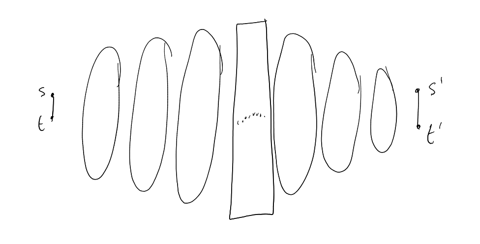
Theorem 4.9 (Alon-Boppana). Assuming that:

$G = (V, E)$ an $(n, d, λ)$ -graph

Then as

n \to \infty

λ \geq 2 \sqrt{d - 1} - O (1) .

Proof 1. Pick edge $s t$ , pick $r \in ℤ_{\geq 0}$ .

$φ : V \to ℝ$ ,

φ (x) = {\begin{matrix} {(d - 1)}^{- i ∕ 2} & if x \in V_{i}, i \leq r \\ 0 & if x \in V_{i}, i > r \end{matrix}

q_{L} (φ) = \frac{⟨ φ, L φ ⟩}{⟨ φ, φ ⟩} ⟨ φ, φ ⟩ = \sum_{i = 0}^{r} \frac{| V_{i} |}{{(d - 1)}^{i}} .

\begin{array}{l} ⟨ φ, L φ ⟩ & = \sum_{x \sim y} {(φ (x) - φ (y))}^{2} \\ = \sum_{i = 0}^{r - 1} e (V_{i}, V_{i + 1}) {(\frac{1}{{(d - 1)}^{i ∕ 2}} - \frac{1}{{(d - 1)}^{(i + 1) ∕ 2}})}^{2} + \frac{e (V_{r}, V_{r + 1})}{{(d - 1)}^{r}} \\ = \sum_{i = 0}^{r - 1} \frac{e (V_{i}, V_{i + 1})}{{(d - 1)}^{i}} {(1 - \frac{1}{\sqrt{d - 1}})}^{2} + \frac{e (V_{r}, V_{r + 1})}{{(d - 1)}^{r}} \end{array}

e (V_{i}, V_{i + 1}) \leq (d - 1) | V_{i} |

\begin{array}{l} ⟨ φ, L φ ⟩ & \leq \sum_{i = 0}^{r - 1} \frac{| V_{i} |}{{(d - 1)}^{i}} {(\sqrt{d - 1} - 1)}^{2} + \frac{| V_{r} |}{{(d - 1)}^{r}} (d - 1) \\ {(\sqrt{d - 1} - 1)}^{2} & = (d - 1) - 2 \sqrt{d - 1} + 1 = d - 2 \sqrt{d - 1} \\ ⟨ φ, L φ ⟩ & \leq (d - 2 \sqrt{d - 1}) \sum_{i = 0}^{r - 1} \frac{| V_{i} |}{{(d - 1)}^{i}} + (d - 1) \frac{| V_{r} |}{{(d - 1)}^{r}} \\ | V_{r} | & \leq (d - 1) | V_{r - 1} | \leq \dots \leq {(d - 1)}^{r - i} | V_{i} | \\ ⟹ \frac{| V_{r} |}{{(d - 1)}^{r}} & \leq \frac{1}{r} \sum_{i = 0}^{r} \frac{| V_{i} |}{{(d - 1)}^{i}} \\ ⟨ φ, L φ ⟩ & \leq (d - 2 \sqrt{d - 1}) \sum_{i = 0}^{r} \frac{| V_{i} |}{{(d - 1)}^{i}} + (2 \sqrt{d - 1}) \frac{| V_{r} |}{{(d - 1)}^{r}} \\ \leq (d - 2 \sqrt{d - 1} + \frac{2 \sqrt{d - 1} - 1}{r + 1}) ⟨ φ, φ ⟩ \\ ⟹ λ_{2} (L) & = \min_{\dim W = 2} \max_{\begin{array}{c} f \in W \\ f \neq 0 \end{array}} \frac{⟨ f, L f ⟩}{⟨ f, f ⟩} \end{array}

Suppose $G$ has 2 deges at distance $> 2 r + 2$ .

$f$ , $f^{'}$ as above. $⟨ f, f^{'} ⟩ = 0$ .

Q_{L} (α f + β f^{'}) = Q_{L} (α f) + Q_{L} (β f^{'}) .

Let $W = span {f, f^{'}}$ .

\begin{array}{l} λ_{2} (L) & \leq \max_{(α, β) \neq (0, 0)} \frac{Q_{L} (α f + β f^{'})}{∥ α f + β f^{'} ∥} \\ \leq \frac{α^{2} Q_{L} (f) + β^{2} Q_{L} (f^{'})}{α^{2} ∥ f ∥ + β^{2} ∥ f^{'} ∥} \\ \leq d - 2 \sqrt{d - 1} + \frac{2 \sqrt{d - 1} - 1}{r + 1} □ \end{array}

Corollary 4.10. For all $d$ , there are finitely many $(n, d, λ)$ -graphs with $λ < 2 \sqrt{d - 1}$ .

$r = c \log n$ .

λ_{n - 1} (A_{G}) \geq 2 \sqrt{d - 1} - O_{d} (\frac{1}{\log n}) .

For Alon-Boppana:

Proof 2. $Tr A^{2 k} = \sum_{x} A^{2 k} (x, x)$ . Note that

# {closed walks of length 2 k in G starting from x} .

is at least

# {closed walks of length 2 k in \prod_{d} starting from 0}

( $\prod_{d}$ is an infinite $d$ -regular tree). The latter is at least

{(d - 1)}^{k} \frac{1}{k + 1} (\binom{2 k}{k}) \approx {(2 \sqrt{d - 1})}^{2 k + o (1)} 2^{2 k} .

\leq \sum_{i = 1}^{n} λ_{i}^{2 k} \leq d^{2 k} + (n - 1) λ^{2 k} .

Exercise: finish details. □

$\min {| λ_{1} (A) | λ_{n - 1} (A)} \geq \dots$

4.1 One-sided expanders

Goal is to find: $G_{n}$ graphs with $n$ vertices, $d$ -regular such that $λ_{n - 1} (A_{G}) \leq λ < d$ .

Reminder: (Friedman) If $G \sim G_{n, d}$ uniform random $d$ -regular graph then

ℙ (G_{n} is (n, d, 2 \sqrt{d - 1} + 𝜀) -graph) \to 1 .

Φ (G_{n}) \geq \frac{λ_{2} ({\tilde{L}}_{G})}{2} = \frac{λ_{2} (L_{G})}{2 d} = \frac{(d - λ_{n - 1} (A_{G}))}{2 d} \geq \frac{1}{2} - \frac{𝜀}{2} > 0 .

Theorem 4.11. Assuming that:

$d = 2 l$ large enough

Then there is

𝜀 = 𝜀_{d} > 0

such that there are

d

-regular graphs (or multi-graphs)

G_{n}

n

vertices with

Φ (G_{n}) \geq 𝜀

for all sufficiently large

n

Graphs $G_{n}$ are as follows:

$V (G_{n}) = [n]$ , $d = 2 l$ .
Take $π_{1}, \dots, π_{l} : [n] \to [n]$ uniform independent permutations.

Set

E (G_{n}) = {{x, π_{i} (x)} : x \in [n], i \in [l]} .

Lemma 4.12. There is $c = c_{d} > 0$ such that

ℙ (G_{n} is d -regular, i.e. G_{n} is simple) \geq c - o (1) .

Lemma 4.13. If $G_{n}$ is $d$ -regular, then there exists $𝜀 = 𝜀_{d} > 0$ such that

ℙ (Φ (G_{n}) < 𝜀) \to 0 .

Proof. If $Φ (G_{n}) < 𝜀$ then there exists $F \subseteq [n]$ , $r = | F | \leq \frac{n}{2}$ , there exists $F^{'}$ , $F \subseteq F^{'}$ and $e (F, F^{'}) = d | F |$ and $| F^{'} | = r + r^{'}$ , $r^{'} = ⌊ 𝜀 r ⌋$ .

ℙ (Φ (G_{n}) < 𝜀) < \sum_{1 \leq r \leq \frac{n}{2}} \sum_{\begin{array}{c} F \subseteq F^{'} \subseteq [n] \\ | F | = r \\ | F^{'} | = r + r^{'} \end{array}} ℙ (π_{i} (F) \subseteq F^{'} for all i \in [l]) .

$ℙ (π_{1} (F) \subseteq F^{'}) = \frac{(\binom{r + r^{'}}{r})}{(\binom{n}{r})}$ .

ℙ \leq \sum_{1 \leq r \leq \frac{n}{2}} \frac{n!}{r! r^{'}! (n - r - r^{'})!} {(\frac{(\binom{r + r^{'}}{r})}{(\binom{n}{r})})}^{l} .

Fact 1: $\frac{(\binom{a}{k})}{(\binom{b}{k})} \leq {(\frac{a}{b})}^{k}$ if $a \leq b$ .

Proof: It is equivalent to

b a \cdot b (a - 1) \dots b (a - k + 1) \leq a b \cdot a (b - 1) \dots a (b - k + 1) .

Compare the product term by term.

Fact 2: $n! \geq {(\frac{n}{e})}^{n}$ . Proof:

e^{n} = \sum_{k \geq 0} \frac{n^{k}}{k!} \geq \frac{n^{n}}{n!} .

Using these:

\frac{n!}{r! r^{'}! (n - r - r^{'})!} \leq \frac{n^{r + r^{'}}}{r! r^{'}!} = \frac{n^{r + r^{'}}}{(r + r^{'})!} (\binom{r + r^{'}}{r}) \leq {(2 e)}^{r + r^{'}} {(\frac{n}{e + e^{'}})}^{r + r^{'}} .

\begin{array}{l} ℙ & \leq \sum_{1 \leq r \leq \frac{n}{2}} {(2 e)}^{r + r^{'}} {(\frac{n}{r + r^{'}})}^{r + r^{'}} {(\frac{r + r^{'}}{n})}^{l r} \\ \leq \sum_{1 \leq r \leq \frac{n}{2}} {(2 e)}^{2 r} {(\frac{(1 + 𝜀) r}{n})}^{r (l - 1 - 𝜀)} \end{array}

Decompose as $\sum_{1 \leq r \leq n ∕ 2} = \sum_{1 \leq r \leq K} + \sum_{K < r \leq n ∕ 2} = S_{1} + S_{2}$ . Choose $𝜀 > 0$ small so that $γ = \frac{1 + 𝜀}{2}$ is small. Choose $l$ large so that $γ^{l - 1 - 𝜀} < \frac{1}{2 {(2 e)}^{2}}$ .

\begin{array}{l} S_{2} & \leq \sum_{K < r \leq \frac{n}{2}} {(2 e)}^{2 r} {(\frac{(1 + 𝜀)}{2})}^{r (l - 1 - 𝜀)} \\ \leq \sum_{K < r \leq \frac{n}{2}} {(\frac{1}{2})}^{r} \\ \leq \frac{1}{2^{K}} \end{array}

Now $S_{1}$ .

\begin{array}{l} S_{1} & \leq \sum_{1 \leq r \leq K} {(2 e)}^{2 r} {(\frac{(1 + 𝜀) r}{n})}^{r (l - 1 - 𝜀)} \\ \leq {(\frac{2 K}{n})}^{l - 2} \sum_{1 \leq r \leq K} {(2 e)}^{2 r} \\ \leq c^{K} {(\frac{K}{n})}^{l} \end{array}

Now let $K = \log \log \log n$ , so this is $\leq O ((\log \log n) n^{- l} {(\log \log \log n)}^{l}) \to 0$ . Also, $S_{1} \leq \frac{1}{2^{K}}$ term goes to $0$ . □

For the lemma about $ℙ (d -regular) \geq c - o (1)$ :

These are the bad things. Use Bonferroni inequalities (the partial sum of inclusion exclusion principle inequalities).

$(n, d, λ)$ -graph

$n$ : number of vertices, $d$ -regular, $λ_{k} (A) \in [- λ, λ]$ , $k \neq n$ .

Ramanujan graph: $(n, d, 2 \sqrt{d - 1})$ -graph.

Petersen $(10, 3, 2 \sqrt{2})$ -graph.
Complete (bipartite), $d = n - 1$ big :(.
Paley $Cay (ℤ ∕ p ℤ, {x^{2} : x \in ℤ ∕ p ℤ, x \neq 0})$ , $p \equiv 1 (m o d 4)$ . $d = \frac{p - 1}{2}$ big :(.

Alon-Boppana: For every $𝜀 > 0$ fixed $d \geq 3$ , there are finitely many $(n, d, 2 \sqrt{d - 1} - 𝜀)$ -graphs.

Bipartite: $(n, d, λ)$ -graph, $n$ vertices, $d$ -regular, $λ_{k} (A) \in [- λ, λ]$ for $k \neq n, 1$ .

Theorem 4.14 (Lubotsky-Phillips-Sanak / Margoulis). Assuming that:

$p$ prime
$d = p + 1$
$n$ arbitrarily large

Then there exists a

(n, d, 2 \sqrt{d - 1})

-graph.

Goal:

Theorem 4.15 (Marcus, Spielman, Srivastava). Assuming that:

$d \geq 3$

Then there are

(n, d, 2 \sqrt{d - 1})

-bipartite graphs for arbitrarily large

n

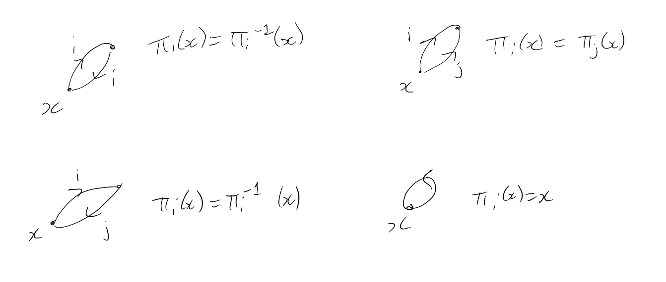
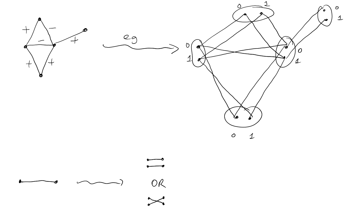
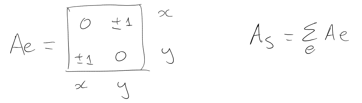
Strategy: Bilu and Linial. Lifts of graphs:

Definition 4.16 (2-lift). A 2-lift of a graph $G = (V, E)$ is a graph $Ĝ = (\hat{V}, Ê)$ with

$x \in V$ $⟹$ $x_{0}, x_{1} \in \hat{V}$ .
$x y \in E$ $⟹$ either $x_{0} y_{0}, x_{1} y_{1} \in Ê$ or $x_{0} y_{1}, x_{1} y_{0} \in Ê$ .

(and no other vertices or edges).

Definition 4.17 (Signing). $S : V \times V \to ℝ$ is a signing of $G$ if

S (x, y) = {\begin{matrix} \pm 1 & if A (x, y) = 1 \\ 0 & if A (x, y) = 0 \end{matrix}

and $S (x, y) = S (y, x)$ (symmetric). So can think of $S$ as a function $E \to {\pm 1}$ .

$A_{S}^{+} (x, y) = A (x, y) 𝟙_{S (x, y) = 1}$ . $A_{S}^{-} (x, y) = A (x, y) 𝟙_{S (x, y) = - 1}$ . Have $A = A_{S}^{+} + A_{S}^{-}$ , $S = A_{S}^{+} - A_{S}^{-}$ .

Lemma 4.18. The eigenvalues of $Ĝ$ are the eigenvalues of $A_{G}$ (old) together with the eigenvalues of $S$ (new).

Proof.

A_{Ĝ_{S}} = (\begin{matrix} A_{S}^{+} & A S_{S}^{-} \\ A_{S}^{-} & A S_{S}^{+} \end{matrix})

Let $A φ = λ φ$ . Then

A_{Ĝ_{S}} (\begin{matrix} φ \\ φ \end{matrix}) = (\begin{matrix} A_{S}^{+} φ + A_{S}^{-} φ \\ A_{S}^{-} φ + A_{S}^{+} φ \end{matrix}) = (\begin{matrix} A φ \\ A φ \end{matrix}) = (\begin{matrix} λ φ \\ λ φ \end{matrix}) = λ (\begin{matrix} φ \\ φ \end{matrix}) .

Let $S η = μ η$ . Now

A_{Ĝ_{S}} (\begin{matrix} η \\ - η \end{matrix}) = (\begin{matrix} A_{S}^{+} η - A_{S}^{-} η \\ A_{S}^{-} η - A_{S}^{+} η \end{matrix}) = (\begin{matrix} S η \\ - S η \end{matrix}) = (\begin{matrix} μ η \\ - μ η \end{matrix}) = μ (\begin{matrix} η \\ - η \end{matrix}) . □

Conjecture 4.19 (Bilu, Linial). If $G$ is $d$ -regular, then there exists a signing $S : E (G) \to {\pm 1}$ whose eigenvalues are in $[- 2 \sqrt{d - 1}, 2 \sqrt{d - 1}]$ .

Theorem 4.20 (Bilu, Linial). Can find signings $S$ with eigenvalues $λ$ satisfying $| λ | = O (\sqrt{d {(\log d)}^{3}})$ .

Theorem 4.21 (Marcusm, Spielman, Srivastava). Assuming that:

$G$ is a $d$ -regular graph

Then there exists a signing with eigenvalues

λ

with

λ \leq 2 \sqrt{d - 1}

Theorem 4.21 implies Theorem 4.15.

Start with $K_{d, d}$ .
Keep applying Theorem 4.21 to find signing.
Build lift with that signing.
2-lift of bipartite graph is bipartite.
Spectrum of adjacency matrix of bipartite graph is symmetric around $0$ . □

Notation. For $π \in Sym (X)$ , let $| π |$ be the number of inversions.

Theorem 4.21: $S \sim Unif ({\pm 1}^{E (G)})$ .

\begin{array}{l} 𝔼_{S} \det (x I - S) & = 𝔼_{S} (\sum_{π \in Sym (X)} {(- 1)}^{| π |} \prod_{y \in V} (x I - S) (y, π (y))) \\ = \sum_{k = 0}^{n} x^{n - k} {(- 1)}^{k} \sum_{\begin{array}{c} T \subseteq V \\ | T | = k \end{array}} \sum_{π \in Sym (T)} 𝔼_{S} ({(- 1)}^{| π |} \prod_{y \in T} (x I - S) (y, π (y))) \end{array}

For $x y \in E$ : $𝔼 S {(x, y)}^{2 k + 1} = 0$ , $𝔼 S {(x, y)}^{2 k} = 1$ .

\begin{array}{l} = \sum_{\begin{array}{c} k = 0 \\ k even \end{array}}^{n} x^{n - k} {(- 1)}^{k} \sum_{\begin{array}{c} M matching \\ of size \leq \frac{k}{2} \end{array}} {(- 1)}^{k ∕ 2} \dots \\ = \sum_{k \geq 0} x^{n - 2 k} {(- 1)}^{k} M_{k} (G) \\ = μ_{G} (x) \end{array}

where

M_{k} (G)

is the number of matchings of size

k

G

$μ_{G} (x)$ is the matching polynomial of $G$ .

Heilman-Lieb-Godsil:

$μ_{G} (x)$ is real rooted for all $G$ .
If $G$ has degree $\leq d$ , then $μ_{G} (x)$ has roots in $[- 2 \sqrt{d - 1}, 2 \sqrt{d - 1}]$ .

Last time, when working on $\det (x I - A_{s})$ , we showed:

Theorem 4.22 (Godsil-Gutman, 80s).

𝔼_{S \sim {\pm 1}} \det (x I - A_{s}) = μ_{G} (x),

where

μ_{G} (x) = \sum_{k \geq 0} x^{n - 2 k} {(- 1)}^{k} m_{k} (G),

where $m_{k} (G)$ is the number of matchings in $G$ with $k$ edges.

Fact: $μ_{G} (x)$ is real rooted.

Theorem 4.23 (Heilman-Lieb, 72). Assuming that:

$G$ is $d$ -regular

Then

maxroot μ_{G} (x) \leq 2 \sqrt{d - 1} .

If only we could say that $maxroot 𝔼_{S} \det (x I - A_{s})$ is an average of $maxroot \det (x I - A_{h})$ , $h \in {\pm 1}^{E}$ . Hopelessly false:

Definition 4.24 (Interlacing). Let $f$ be a real rooted polynomial of degree $n$ with roots $α_{1}, \dots, α_{n}$ and $g$ a real rooted polynomial of degree $n - 1$ with roots $β_{1}, \dots, β_{n - 1}$ . We say $g$ interlaces $f$ if

α_{1} \leq β_{1} \leq α_{2} \leq \dots \leq β_{n - 2} \leq α_{n - 1} \leq β_{n - 1} \leq α_{n} .

Example. If $f$ is real rooted, then so is $f^{'}$ , and also $f^{'}$ interlaces $f$ .

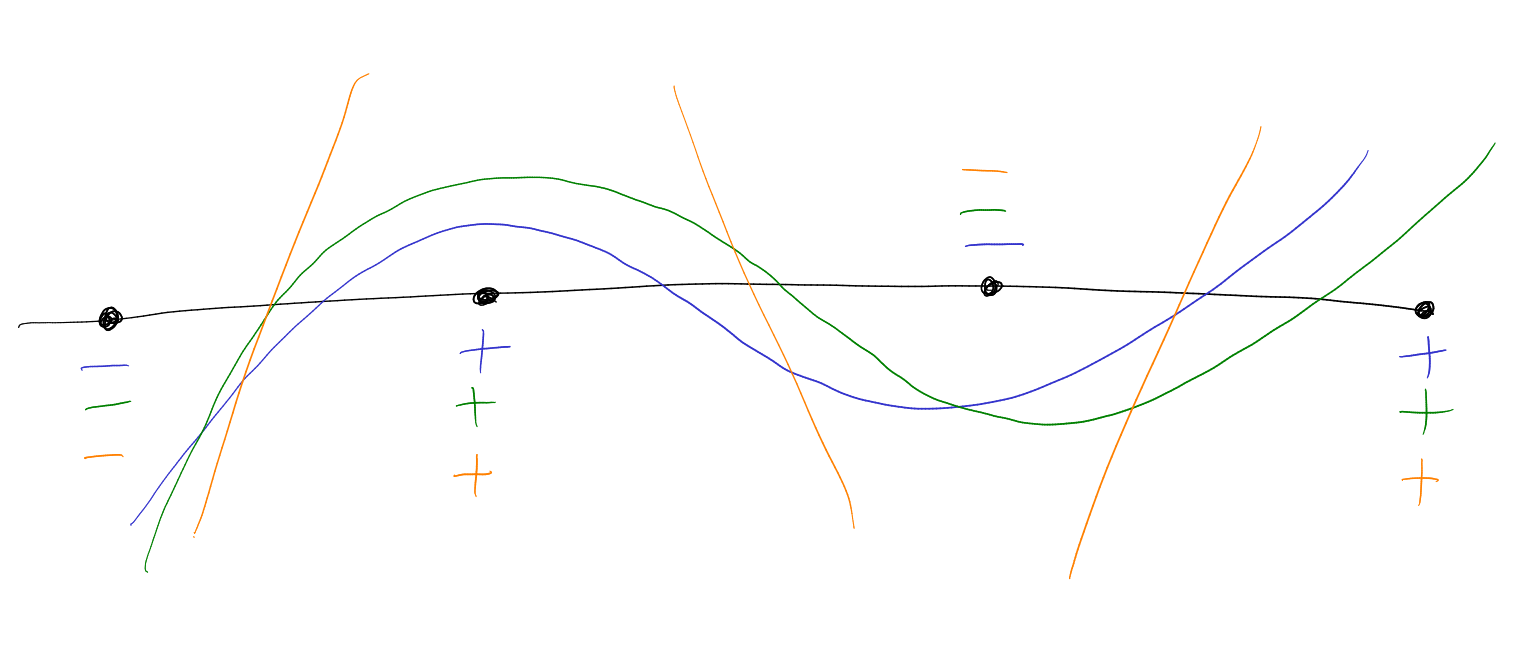
Definition 4.25 (Common interlacement). We say that real rooted polynomials $f$ , $g$ of degree $n$ have a common interlacement if there is a polynomial $h$ of degree $n + 1$ such that $f$ and $g$ both interlace $h$ . In other words, if the roots of $f$ and $g$ are $α_{1} \leq \dots α_{n}$ and $β_{1} \leq \dots \leq β_{n}$ respectively, then they have a common interlacement if and only if there are some $γ_{0} \leq \dots \leq γ_{n}$ such that

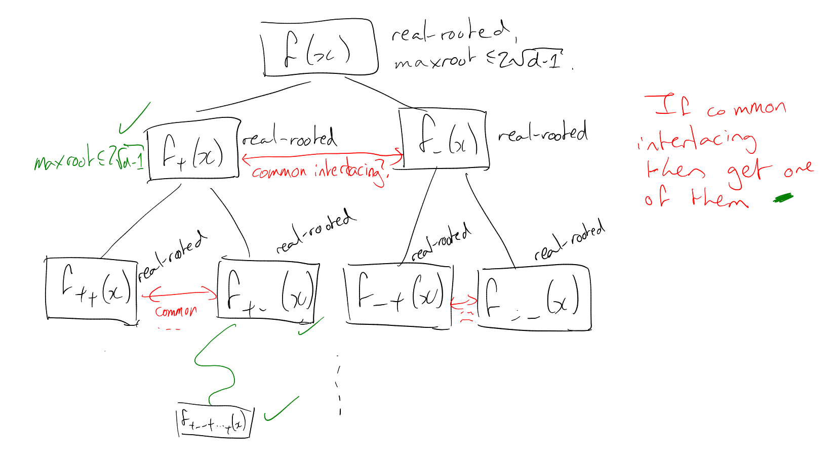
γ_{0} \leq α_{1}, β_{1} \leq γ_{1} \leq α_{2}, β_{2} \leq γ_{2} \leq \dots \leq γ_{n - 1} \leq α_{n}, β_{n} \leq γ_{n} .

Theorem 4.26 (Fell 80). Assuming that:

$f$ , $g$ are real rooted
both degree $n$ , monic

Then

f

and

g

have a common interlacing if and only if every convex combination of

f

and

g

are real rooted.

Proof. Assume $f$ and $g$ without repeated or common roots (general case requires more work and details checking).

$\Leftarrow$ Let $h_{t} (x) = t f (x) + (t - 1) g (x)$ for $t \in (0, 1)$ . We know these are real rooted, and waht to show that $f$ , $g$ have a common interlacement. Let $λ_{i} (t)$ be the $i$ -th root of $h_{t} (x)$ . $λ_{i} (t)$ includes $(λ_{i} (0), λ_{i} (1)) \subseteq ℝ$ .
Claim: $(λ_{I} (0), λ_{I} (1))$ are disjoint.

Suppose not. Let $λ_{k}$ be a root of $f$ and $λ_{k} \in (λ_{I} (0), λ_{I} (1))$ . So there exists $t \in (0, 1)$ such that $λ_{I} (t) = λ_{k}$ .

$h_{t} (λ_{k}) = 0 = t f (λ_{k}) + (1 - t) g (λ_{k}),$

so $g (λ_{k}) = 0$ , contradiction as we assumed no common roots.
$\Rightarrow$

The dots represent the roots of the polynomial that interlaces them. By monicness, we get the blue and green $+$ s and $-$ s. Then get the orange ones, and use intermediate value theorem. □

Corollary 4.27. Assuming that:

$f$ , $g$ are real rooted of degree $n$
have a common interlacing

Then for all

t \in [0, 1]

\min {maxroot (f), maxroot (g)} \leq maxroot (t f (x) + (1 - t) g (x)) .

Approach to Theorem 4.21:

$f (x) = 𝔼_{S \in {\pm 1}^{E}} \det (x I - A_{s})$ , $| E | = m$ . For $h_{1}, \dots, h_{k} \in {\pm 1} = {+, -}$ , then

f_{h_{1}, \dots, h_{k}} (x) = 𝔼_{s_{k + 1}, \dots, s_{m} \in {\pm 1}} (\det (x I - A_{s}) | s_{1} = h_{1}, \dots, s_{k} = h_{k}) .

“Method of interlacing families of polynomials”

Theorem 4.28 (Marcus, Spielman, Srivastava (real rooted)). For every $ρ_{1}, \dots, ρ_{m} \in [- 1, 1]$ the following polynomial is real rooted

χ_{ρ_{1}, \dots, ρ_{m}} (x) = \sum_{S \in {\pm 1}^{m}} \det (x I - A_{s}) \prod_{J : s_{J} = 1} (\frac{1 + ρ_{J}}{2}) \prod_{J : S_{J} = - 1} (\frac{1 - ρ_{J}}{2}) .

Theorem 4.28 implies Theorem 4.21:

f_{h_{1}, \dots, h_{k}} (x) = χ_{h_{1}, \dots, h_{k}, 0, 0, \dots, 0} (x) .

μ_{G} (x) = χ_{0, \dots, 0} (x) .

t f_{h_{1}, \dots, h_{k}, 1} (x) + (1 - t) f_{h_{1}, \dots, h_{k}, - 1} (x) = χ_{h_{1}, \dots, h_{k}, 2 t - 1, 0, \dots, 0} (x) .

Theorem 4.29 (Marcus, Spielman, Srivastava (matrix)). Assuming that:

$r_{1}, \dots, r_{m} \in ℝ^{n}$ are independent random vectors, whose support has $\leq 2$ points

Then

𝔼 \det (x I - \sum_{j = 1}^{m} r_{j} r_{j}^{⊤})

is real rooted.

Theorem 4.29 implies Theorem 4.28:

$χ_{ρ_{1}, \dots, ρ_{m}} (x)$ is

𝔼 \det (x I - A_{s}) .

$𝔼 \det (x I - A_{s})$ is real rooted if and only if $𝔼 \det ((x + d) I - A_{s})$ is real rooted. This equals

𝔼 \det (x I + (d I - A_{s})) .

Note

d I - A_{S} = \sum_{x \sim y} (e_{x} + S (x, y) e_{y}) {(e_{x} + S (x, y) e_{y})}^{⊤} .

Done.

Definition 4.30 (Real stable). A polynomial $p (z_{1}, \dots, z_{n}) \in ℝ [z_{1}, \dots, z_{n}]$ is real stable if $p (z_{1}, \dots, z_{n}) \neq 0$ for all $(z_{1}, \dots, z_{n}) \in H^{n}$ , $H = {z \in ℂ | Im z > 0}$ .

Notice that for a single variable, $p (z)$ is real stable if and only if real rooted.

Example. $1 - z_{1} z_{2}$ .

Proposition 4.31 (Stable iff real rooted). $p (z_{1}, \dots, z_{n})$ is real stable if and only if for all $ℝ_{\geq 0}^{n}$ , $b \in ℝ^{n}$ , the polynomial $t \mapsto p (a t + b)$ is real rooted.

Proof.

$\Rightarrow$ If $p$ not stable, then there exists $z_{0}, \dots, z_{n} \in H$ with $p (z_{1}, \dots, z_{n}) = 0$ , $z_{j} = b_{j} + i a_{j}$ , $a_{j} > 0$ . Then $p (a i + b) = 0$ , $t = i$ .
$\Leftarrow$ Suppose $\exists a \in ℝ_{\geq 0}^{n}$ , $b \in ℝ^{n}$ , $t \in ℂ ∖ ℝ$ with $p (a t + b) = 0$ . Assume $Im t > 0$ . $z_{j} + a_{j} t + b_{j} \in H$ . $p (z_{1}, \dots, z_{n}) = p (a t + b) = 0$ .

□

Proposition 4.32 (Stability of real stable). Assuming that:

$p (z_{1}, \dots, z_{n})$ is real stable

Then the following are also:

$p (z_{σ (1)}, \dots, z_{σ (n)})$ , $σ \in S_{n}$ .
$p (a z_{1}, z_{2}, \dots, z_{n})$ , $a \in ℝ_{\geq 0}$ .
$p (z_{2}, z_{2}, z_{3}, \dots, z_{n})$ .
$p (c, z_{2}, \dots, z_{n})$ , $c \in H \cup ℝ$ .
$z_{1}^{d_{1}} p (- \frac{1}{z_{1}}, z_{2}, \dots, z_{n})$ .
$\partial_{z_{1}} p (z_{1}, \dots, z_{n})$ .
$MAP (p (z_{1}, \dots, z_{n}))$ . $MAP (z_{1} z_{2} + z_{2} z_{3}^{2} + 2 z_{1} z_{4} + z_{2} z_{3}^{2}) = z_{1} z_{2} + 2 z_{1} z_{4}$ .
If $p, q$ are real stable, then so is $p q$ .

Proposition 4.33 (Mother of all stable polynomials). Assuming that:

$B \in ℝ^{d \times d}$ symmetric matrix
$A_{1}, \dots, A_{m} \in ℝ^{d \times d}$ positive semi definite

Then

\det (B + z_{1} A_{1} + \dots + z_{n} A_{n})

is real stable.

Proof. Let $a \in ℝ_{\geq 0}^{n}$ , $b \in ℝ^{n}$ . Assume positive definite instead of positive semi definite.

\begin{array}{l} \det (B + \sum_{j = 1}^{n} (a_{j} t + b_{j}) A_{j}) = \det (\underset{= : A}{\underset{⏟}{(\sum_{j = 1}^{n} a_{j} A_{j})}} t + \underset{= : C}{\underset{⏟}{(\sum_{j = 1}^{n} b_{j} A_{j} + B)}}) \end{array}

$A$ is positive definite, and $C$ is symmetric. So

\begin{array}{l} = \det (A t + C) \\ = \det (A^{\frac{1}{2}} (t I + A^{- \frac{1}{2}} C A^{- \frac{1}{2}}) A^{\frac{1}{2}}) \\ = \det A \det (t I + A^{- \frac{1}{2}} C A^{- \frac{1}{2}}) \end{array}

The roots are eigenvalues of a real symmetric matrix, hence real. □

Proof of Theorem 4.29. Say $r_{j}$ equals $r_{j}^{+}$ with probability $p_{j}^{+}$ , and equals $r_{j}^{-}$ with probability $p_{j}^{-}$ . We will use Cauchy Binet:

\det (A B) = \sum_{\begin{array}{c}  \end{array}} \det (A_{S \times [n]}) \det (B_{[n] \times C}) T O D O

\begin{array}{l} p (z_{1}, \dots, z_{n}) & = 𝔼 \det (\sum_{j = 1}^{n} z_{j} r_{j} r_{j}^{⊤}) \\ = 𝔼 \sum_{\begin{array}{c} S \subseteq [m] \\ | S | = n \end{array}} \det (\sum_{j \in S} z_{j} r_{j} r_{j}^{⊤}) \\ = 𝔼 \sum_{\begin{array}{c} S \subseteq [m] \\ | S | = n \end{array}} (\prod_{j \in S} z_{j}) \det (\sum_{j \in S} r_{j} r_{j}^{⊤}) \end{array}

\det (𝔼 \sum_{j = 1}^{n} z_{j} r_{j} r_{j}^{⊤}) = \det (\sum_{j = 1}^{n} z_{j} 𝔼 r_{j} r_{j}^{⊤})

is real stable since $𝔼 r_{j} r_{j}^{⊤} \geq 0$ is a covariance matrix.

\begin{array}{l} = \det (\sum_{j = 1}^{m} z_{j} (p_{j}^{+} r_{j}^{+} {(r_{j}^{+})}^{⊤} + p_{j}^{-} r_{j}^{-} {(r_{j}^{-})}^{⊤})) \\ = \sum_{\begin{array}{c} S \subseteq [m] \\ | S | = n \end{array}} (\prod_{j \in S} z_{j}) \sum_{n \in {\pm 1}^{S}} \det (p_{j}^{h (j)} r_{j}^{h (j)} {(r_{j}^{h (j)})}^{⊤}) + “terms with squares” \end{array}

So the earlier thing is real stable. So

𝔼 \det (\sum_{j = 1}^{m} z_{j} r_{j} r_{j}^{⊤})

is real stable. So

𝔼 \det (\sum_{j = 1}^{m} z_{j} r_{j} r_{j}^{⊤} + \sum_{j = 1}^{m} x_{j} e_{j} e_{j}^{⊤})

is real stable. Take $z_{j} = - 1$ , $x_{j} = x$ . Then

𝔼 \det (x I - \sum_{j = 1}^{m} r_{j} r_{j}^{⊤})

is real stable. □

Theorem 4.34 (Godsil). Assuming that:

$G$ is $d$ -regular
$λ_{1} \leq \dots \leq λ_{n}$ are the roots of $μ_{G} (x)$

Then

\sum_{k = 1}^{n} λ_{k}^{l} = \sum_{a} W_{a}^{l} (G),

where $W_{a}^{l} (G)$ is the number of closed walks of length $l$ from $a$ in the path tree $T_{a} (G)$ of $G$ .

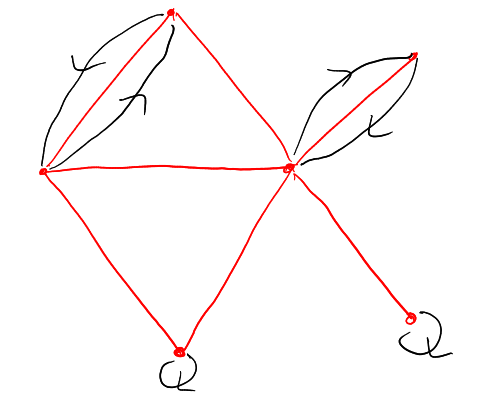
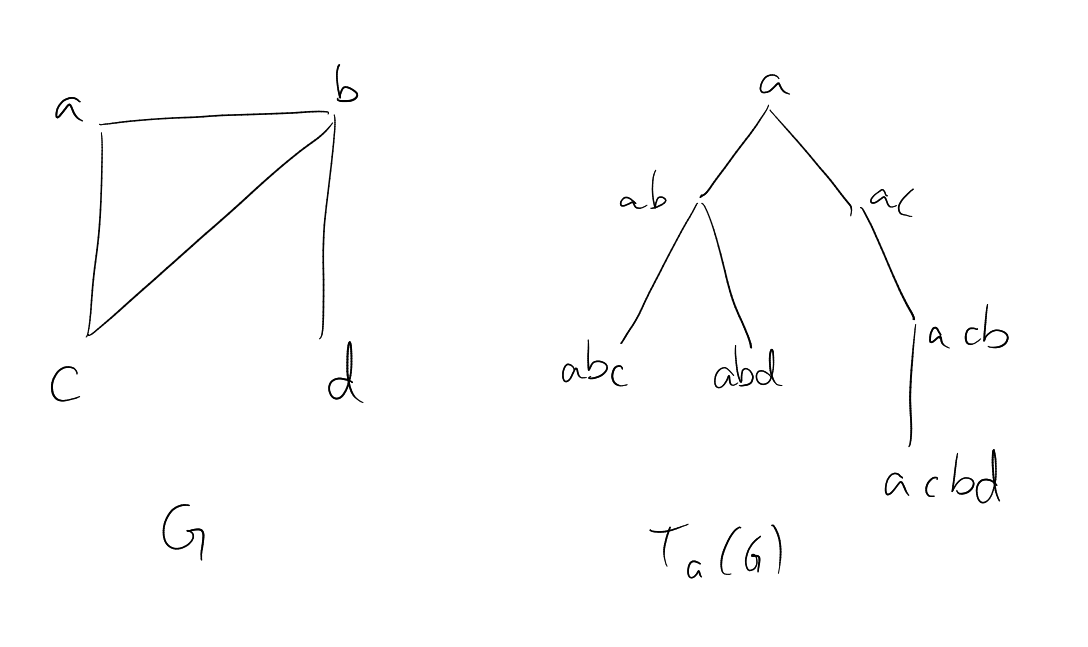
Definition 4.35 (Path tree). Example: $T_{a} (G)$

Proof of ?? implies Theorem 4.23. $W_{a}^{l} (G) \leq W_{a}^{l} (\prod_{d}) \leq {(2 \sqrt{d - 1} + o_{l} (1))}^{l}$ .

$λ_{n}^{l} \leq \sum λ_{k}^{l} = \sum_{a} W_{a}^{l} (G) \leq n {(2 \sqrt{d - 1} + o_{l} (1))}^{l}$ .

$λ_{n} \leq n^{\frac{1}{l}} (2 \sqrt{d - 1} + o_{l} (1))$ .

Take $l \to \infty$ . □

Proof of ??. $μ_{G}^{'} (x) = \sum_{a} μ_{G - a} (x)$ Hence

\begin{array}{l} \sum_{a} \sum_{k \geq 0} x^{n - 1 - 2 k} {(- 1)}^{k} m_{k} (G - a) & = \sum_{k \geq 0} (n - 2 k) x^{n - 1 - 2 k} {(- 1)}^{k} m_{k} (G) \\ = μ_{G}^{'} (x) \end{array}

\begin{array}{l} μ_{G} (x) & = x μ_{G - a} (x) - \sum_{b \sim a} μ_{G - a - b} (x) \\ m_{k} (G) & = m_{k} (G - a) + \sum_{b \sim a} m_{k - 1} (G - a - b) \\ x^{n - 2 k} {(- 1)}^{k} m_{k} (G) & = x \cdot x^{n - 1 - 2 k} {(- 1)}^{k} m_{k} (G - a) - \sum_{b \sim a} x^{n - 2 - 2 (k - 1)} {(- 1)}^{k - 1} m_{k - 1} (G - a - b) \\ \sum_{a} \frac{μ_{G - a} (x)}{μ_{G} (x)} & = \frac{μ_{G}^{'} (x)}{μ_{G} (x)} \\ = \sum_{j = 1}^{n} \frac{1}{x - λ_{j}} \\ = \frac{1}{x} \sum_{j = 1}^{n} \frac{1}{1 - \frac{λ_{j}}{x}} \\ = \frac{1}{x} \sum_{j = 1}^{n} \sum_{l \geq 0} \frac{λ_{j}^{l}}{x^{l}} \\ = \frac{1}{x} \sum_{l \geq 0} \frac{\sum_{j} λ_{j}^{l}}{x^{l}} \end{array}

Claim:

\frac{μ_{G - a} (x)}{μ_{G} (x)} = \frac{1}{x} \sum_{l \geq 0} \frac{W_{a}^{l} (G)}{x^{l}}

\begin{array}{l} \frac{μ_{G - a} (x)}{μ_{G} (x)} & = \frac{μ_{G - a} (x)}{x μ_{G - a} (x) - \sum_{b \sim a} μ_{G - a - b} (x)} \\ = \frac{1}{x} \frac{1}{1 - \frac{1}{x} \sum_{b \sim a} \frac{μ_{G - a - b} (x)}{μ_{G - a} (x)}} \\ = \frac{1}{x} \cdot \sum_{k \geq 0} {(\frac{1}{x} \sum_{b \sim a} \frac{μ_{G - a - b} (x)}{μ_{G - a} (x)})}^{k} \\ = \frac{1}{x} \sum_{k \geq 0} \frac{1}{x^{k}} {(\sum_{b \sim a} \frac{1}{x} \sum_{l \geq 0} \frac{W_{b}^{l} (G - a)}{x^{l}})}^{k} \\ = \frac{1}{x} \sum_{k \geq 0} \frac{1}{x^{2 k}} (\sum_{b_{1} \sim a} \sum_{l_{1} \geq 0} \frac{W_{G}^{l_{1}} (G - a)}{x^{l_{1}}}) \dots (\sum_{b_{k} \sim a} \sum_{l_{k} \geq 0} \frac{W_{b_{k}}^{l_{k}} (G - a)}{x^{l_{k}}}) \\ = \frac{1}{x} \sum_{l \geq 0} \frac{W_{a}^{l} (G)}{x^{l}} \end{array}

Why? A tree-like walk in $W_{a}^{l} (G)$ that visits $a$ exactly $k$ times is determined by:

A sequence $b_{1}, \dots, b_{k}$ of neighbours of $a$ .
A sequence $γ_{1}, \dots, γ_{k}$ of walks in $T_{b_{i}}^{l_{i}} (G - a)$ where $2 k + l_{1} + \dots + l_{k} = l$ .

□

Index

Contents

1 Setting

2 Graphs and some of their matrices

2.1 Irregular graphs

3 Expansion and Cheeger inequality

Fiedler’s Algorithm

4 Loewner order

Vertex expansion

Why aren’t Cayley graphs of abelian groups expanders?

4.1 One-sided expanders

Index