Spectral Graph Theory
Lectured by Victor Souza

Contents

1Setting
2Graphs and some of their matrices
2.1Irregular graphs
3Expansion and Cheeger inequality
4Loewner order
4.1One-sided expanders
Index

“linear algebraic methods in combinatorics”

1 Setting

Ω a set (finite), f : Ω → ℂ, l2(Ω) := {f : Ω → ℂ|∑ ⁡ x|f(x)|2 < ∞}.

This generalises subsets: given S ⊆Ω, can consider 𝟙S : Ω → ℂ (where x↦1 for x ∈ S, and x↦0 otherwise).

When S contains only a single element, we may use the shorthand 𝟙x = 𝟙{x}.

l2(Ω) is a ℂ-vector space, equipped with the inner product ⟨∙,∙⟩ : l2(Ω) × l2(Ω) → ℂ defined by

⟨f,g⟩:= ∑ x∈Ωf(x)¯g(x),

and a norm ∥f∥22 := ⟨f,f⟩ = ∑ ⁡ x|f(x)|2.

Matrix over Ω: M : Ω ×Ω → ℂ. M(x,y) = Mx,y is the x,y entry. M acts on l2(Ω): for f ∈ l2(Ω), Mf ∈ l2(Ω) is given by (Mf)(x) = ∑ ⁡ yM(x,y)f(y). M(αf + βg) = αMf + βMg (M is a linear map).

Given M, N, can calculate

(MNf)(X) = ∑ y ∑ zM(x,z)N(z,y)f(y),

so define (MN)(x,y) = ∑ ⁡ zM(x,z)N(z,y), so that the formula (MNf)(x) = ∑ ⁡ y(MN)(x,y)f(y) holds.

Eigenthings: for M : Ω ×Ω → ℂ, we say that λ ∈ ℂ is an eigenvalue with eigenfunction φ≠0 if Mφ = λφ.

Definition 1.1 (Hermitian). M is Hermitian if M = MH, where MH(x,y) = M(y,x)¯.

If M is Hermitian, then ⟨Mf,g⟩ = ⟨f,Mg⟩.

Theorem 1.2 (Spectral theorem for Hermitian matrices). Assuming that:

  • Ω finite

  • M : Ω ×Ω → ℂ Hermitian

  • |Ω| = n

Then there exist λ1,…,λn ∈ ℝ and φ1,…,φ)n ∈ l2(Ω) non-zero such that
  • (1)
    Mφi = λiφi
  • (2)
    ⟨φi,φj⟩𝟙i = j
  • (3)
    M = ∑ ⁡ i=1nλφiφiH
  • (4)
    there exists U orthogonal such that UMUH = diag ⁡ (λi)
  • (5)
    if M is real, then can take φ to be real (φ : Ω → ℝ)

Lemma 1.3. Any M has an eigenpair (λ,φ).

Proof. Want Mf = zf for some z ∈ ℂ. So want (zI − M)f = 0 to have a non-trivial solution f≠0. This happens if and only if zI − M is singular, which happens if and only if det ⁡ (zI − M) = 0.

z↦det ⁡ (zI − M) is a degree n polynomial in ℂ (degree n since the leading term is zn), so the fundamental theorem of algebra shows that there exists λ ∈ ℂ such that det ⁡ (λI − M) = 0. □

Lemma 1.4. Assuming that:

Then all eigenvalues are real

Proof.

λ¯⟨φ,φ⟩ = ⟨λφ,φ⟩ = ⟨Mφ,φ⟩ = ⟨φ,Mφ⟩ = ⟨φ,λφ⟩ = λ⟨φ,φ⟩

Since φ≠0, ⟨φ,φ⟩ = ∥φ∥2 > 0, hence λ = λ¯, i.e. λ ∈ ℝ. □

Lemma 1.5. Assuming that:

  • λi≠λj are eigenvalues of M with eigenvectors φi, φj

Then ⟨φi,φj⟩ = 0.

Proof.

λi⟨φi,φj⟩ = ⟨Mφi,φj⟩ = ⟨φi,Mφj⟩ = λj⟨φi,φj⟩

Since we assumed λi≠λj, this gives ⟨φi,φj⟩ = 0. □

Lemma 1.6. Assuming: - M is real symmetric - λ is an eigenvalue Then: there exists g : Ω → ℝ such that Mg = λg.

Proof. Let φ = f + ig. Then Mφ = Mf + iMg = λφ = λf + iλg. Hence Mf = Mλ and Mg = λg. So either f or g works. □

Notation. For f,g ∈ l2(Ω), fgH denotes the matrix (fgH)(x,y) = f(x)g¯(y).

“(fgH)h = fgHh = f⟨g,h⟩”

Proof of Spectral theorem for Hermitian matrices. Using the above lemmas, can find λn ∈ ℝ and φi : Ω → ℂ non-zero such that Mφn = λnφn and ∥φn∥ = 1.

Then let M′ = M − λnφnφnH. l2(Ω) = span ⁡ (φn) ⊕ span ⁡ (φn)⊤ ⁡. Then check that M′ acts on span ⁡ (φn)⊤ ⁡ and use induction. □

Theorem 1.7 (Courant-Fischer-Weyl Theorem). Assuming: - M : Ω ×Ω → ℝ symmetric - eigenvalues λ1 ≤… ≤ λn Then:

λk = min ⁡ W≤l2(Ω) dim⁡ ⁡ W=k max ⁡ f∈W f≠0 ⟨f,Mf⟩ ⟨f,f⟩ = Fk.

Definition 1.8 (Rayleigh quotient). ⟨f,Mf⟩ ⟨f,f⟩ is called the Rayleigh quotient.

Proof. Let W′ = span ⁡ (φ1,… ⁡ ,φk). Note

Fk ≤ max ⁡ f∈W f≠0 ⟨f,Mf⟩ ⟨f,f⟩ .

For f ∈ W, f = ∑ ⁡ i=1kαiφi, so

⟨f,Mf⟩ ⟨f,f⟩ = ∑ i=1kαi2λi ∑ i=1kαi2 ≤ λk ∑ i=1kαi2 ∑ i=1kαi2 = λk.

So Fk ≤ λk.

Now suppose W is a subspace with dim⁡W = k. Let V = span ⁡ (φk,… ⁡ ,φn), and note ÷ V = n − k + 1. Note

dim⁡(V ∩ W) = dim⁡V + dim⁡W −dim⁡(V + W) ≥ k + (n − k + 1) − n = 1.

So for all such W, there exists f ∈ V ∩ W, f≠0 such that f = ∑ ⁡ i≥kαiφi. Then

⟨f,Mf⟩ = ∑ i≥kαi2λ i ≥ λk ∑ i≥kαi2 = λ k⟨f,f⟩,

so Fk ≥ λk. □

Notation 1.9. Define QM : l2(Ω) → ℂ by QM(f) = ⟨f,Mf⟩ = ∑ ⁡ x,yf(x)M(x,y)f(y).

Define qm(f) = QM(f) QI(f) .

λ1(M) = min ⁡ f≠0qM(f) and it is attained only on

Lemma 1.10. eigenfunctions of λ1.

Proof. Let f = ∑ ⁡ iαiφi and Mf = ∑ ⁡ iαiλiφi. Then

QM(f) = ⟨f,Mf⟩ ∑ i,jαiαjλi⟨φi,φj⟩ = ∑ iαi2λ i

and

q M (f) = ∑ iαi2λi ∑ iαi2 ≥ λi.

Equality occurs here if and only if ∑ ⁡ i(λ1 − λi)αi2 = 0. So αi = 0 whenever λi > λ1. □

Assuming:

Lemma 1.11. - φ1 is an eigenfunction of λ1. Then: λ2(M) = min ⁡ f⊥φ1 f≠0 qM(f), and it is attained only on eigenfunctions of λ2(M).

Proof.

q M (f) = ∑ iαi2λi ∑ iαi2 ≥ α12λ1 + (∑ i≥2αi2) λ2 ∑ iαi2 .

So

min ⁡ f⊥φi f≠0 qM(f) ≥ λ2.

Deal with the equality case similarly to before. □

In general:

λk(M) = min ⁡ f⊥φ1,… ⁡ ,φk−1 f≠0 qM(f).

(and equality case is similar to before). Also,

λn(M) = max ⁡ f≠0qM(f) λn−k(M) = max ⁡ f⊥φn,… ⁡ ,φn−k+1 f≠0 qM(f)

(and equality case is similar to before).

2 Graphs and some of their matrices

Graph G = (V,E): set of vertices V , |V | = n, E is a set of (unordered) pairs of vertices.

Definition 2.1 (Adjacency matrix). The adjacency matrix of a graph G is the matrix AG : V × V → ℝ defined by

AG(x,y) = { 1 {x,y}∈ E(G) 0{x,y}∉E(G)

Definition 2.2 (Degree matrix). The degree matrix of a graph G is the matrix DG : V × V → ℝ defined by

DG(x,y) = { deg⁡(x) x = y 0 otherwise

Definition 2.3 (Laplacian matrix). The Laplacian matrix of a graph G is defined by LG = D −A.

We can now calculate:

QA(f) = ∑ x,yf(x)A(x,y)f(y) = 2∑ x∼yf(x)f(y) QD(f) = ∑ x,yf(x)D(x,y)f(y) = ∑ xf(x)2 deg⁡(x) = ∑ xf(x)2 ∑ yA(x,y) = ∑ x,yf(x)2A(x,y) = 1 2∑ x,y(f(x)2 + f(y)2)A(x,y) = ∑ x∼y(f(x)2 + f(y)2) QL(f) = QD−A(f) = QD(f) −QA(f) = ∑ x∼y(f(x)2 + f(y)2 − 2f(x)f(y)) = ∑ x∼y(f(x) − f(y))2 ≥ 0

Corollary 2.4. For any graph G, LG is a positive semi definite matrix with eigenvector 1, which has eigenvalue 1.

Proof. Since QL(f) = ∑ ⁡ x∼y(f(x) − f(y))2, we see that QL(f) ≥ 0, with equality when f is constant. □

Proposition 2.5. λ2(Lg) > 0 if and only if G is connected. λk(LG) = 0 if and only if G has at least k connected components.

Proof.

λ2 = min ⁡ f⊥1 f≠0 ∑ x∼y(f(x) − f(y))2 ⟨f,f⟩ ≥ 0

Equality happens if and only if QL(f) = 0, which happens if and only if f is constant on connected components. The dimension of {f : constant on connected components} is the number of connected components of G.

TODO? □

TODO

TODO

2.1 Irregular graphs

A, D, L = D − A, QL(f) = ∑ ⁡ x∼y(f(x) − f(y))2, qL(f) = ∑ ⁡ x∼y(f(x)−f(y))2 ∑ ⁡ xf(x)2 .

QL(f) = ⟨f,Lf⟩ = ⟨,(D − A)f⟩ = ⟨f,(2D − (D + A))f⟩ = ⟨f,2Df⟩−⟨f,(D + A)f⟩

When G is d-regular,

L~ G = 1 dLG = I −1 dAG,

λi(L~G ∈ [0,2].

q L~ (f) = ∑ x∼y(f(x) − f(y))2 ∑ xd(x)f(x)2 = 2 −∑ x∼y(f(x) + f(y))2 ∑ xd(x)f(x)2 .

Want M such that qM(f) equals the expression above. Recall qM(f) = ⟨f,Mf⟩ ⟨f,f⟩ . But the above expression is ⟨f,Mf⟩ ⟨f,Df⟩.

Let D1 2 (x,y) = 𝟙x = y d(x). Assume d(x) ≥ 1 for all x ∈ G. Note

q M (D1 2 f) = ⟨D1 2 f,MD1 2 f⟩ ⟨D1 2 f,D1 2 f⟩ = ⟨f,D1 2 MD1 2 f⟩ ⟨f, Df⟩.

Want D1 2 MD1 2 = L = D − A. Define

L~ G = D−1 2 (D − A)D−1 2 = I − D−1 2 AD−1 2 .

So

L~ G = { 1 if x = y − 1 d(x)d(y) if x≠y and x ∼ y 0 if x≠y and x⁄ ∼ y

Also,

q L~G (D1 2 f) = ∑ x∼y(f(x) − y(y))2 ∑ xd(x)f(x)2 .

We have

λk(L~G) = min ⁡ dim⁡ ⁡ W=K max ⁡ f∈W f≠0 qL~G(D1 2 f).

3 Expansion and Cheeger inequality

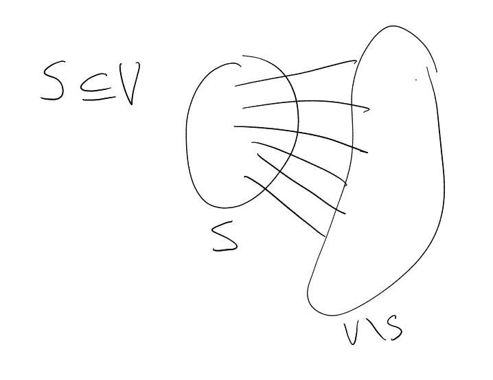
Assume G is d-regular. Write G = (V,E).

PIC

Definition 3.1 (Expansion). Given a d-regular graph G and S ⊆ V , the expansion of S is

Φ(S) := e(S,V ∖ S) d|S| .

Note that 0 ≤Φ ≤ 1, for example because

Φ (S) = ℙ x∼U(S) y∼N(x) (y∉S).

Definition 3.2 (Edge expansion). The (edge) expansion of a cut (S,V ∖ S) is defined as

Φ(S,V ∖ S) := max ⁡ {Φ(S),Φ(V ∖ S)} = e(S,V ∖ S) dmin ⁡ {|S|,|V ∖|}.

Definition 3.3 (Edge expansion of a graph). The edge expansion of a graph is

Φ(G) := min ⁡ S⊆V ∅≠S≠V Φ(S,V ∖S) = min ⁡ S⊆V 0<|S|<|V |∕2 Φ(S).

Theorem 3.4 (Cheeger’s inequality). Assuming that:

  • G be d-regular

Then
λ2(L~G) 2 ≤Φ(G) ≤ 2λ2(L~G).

Consider 𝟙S : V → ℝ, where 𝟙S(x) = 1 if x ∈ S and 𝟙S(x) = 0 otherwise. Then

QL(𝟙S) = ∑ x∼y(𝟙S(x) −𝟙S(y))2 = e(S,V ∖ S) qL~(𝟙S) = e(S,V ∖ S) d|S| = Φ(S)

Recall

λ2(L~G) = min ⁡ dim⁡ ⁡ W=2 max ⁡ f∈W f≠0 qL~G(f).

We pick W = span ⁡ {𝟙S,𝟙V ∖ S}. Note

λ2(L~G) ≤ max ⁡ α,β (α,β)≠(0,0) qL~G(α𝟙S + β𝟙V ∖ S) ≤ max ⁡ α,β2max ⁡ {qL~(G)(α𝟙S),qL~G(β𝟙V ∖ S)}

Lemma 3.5. Assuming that:

  • M is symmetric positive semi-definite

  • ⟨f,g⟩ = 0

Then
q M (f + g) ≤ 2max ⁡ {qM(f),qM(g)}.

Proof. Let λi, φi such that f = ∑ ⁡ iλiφi and g = ∑ ⁡ iβiφi. Then

q M (f + g) = ∑ iλi(αi + βi)2 ∥f + g∥2 ≤ ∑ iλi(2αi2 + 2βi2) ∥f∥2 + ∥g∥2 .

Then

qM(f + g) ≤ 2 (∑ iλiαi2 + ∑ iλiβi2 ∥f∥2 + ∥g∥2 ) = 2 (qM (f)∥f∥2 + qM(g)∥g∥2 ∥f∥2 + ∥g∥2 ) ≤ 2max ⁡ {qM(f),qM(g)}□

Proof of left inequality in Cheeger’s inequality. λ2 ≤ 2max ⁡ {Φ(S),Φ(V ∖ S)} = 2Φ(S,V ∖ S). Then minimise over all S, to get λ2 ≤ 2Φ(G). □

Recall that

Φ (S) = qL~G(𝟙S)

and

Φ (G) = min ⁡ S⊆V 1≤|S|≤|V |∕2 qL~G(𝟙S).
Fiedler’s Algorithm

Input: G,φ : V → ℝ.

Output: The cut.

Running time: O(|V |log⁡|V | + |E|).

Lemma 3.6. Assuming that:

  • ψ : V → ℝ

  • ⟨ψ,1⟩ = 0

  • let (S,V ∖ S) = Fiedler ⁡ (G,ψ)

Then
Φ (S,V ∖ S) ≤ 2qL~G(ψ).

If ψ : V → ℝ, call a cut ({x : ψ(x) ≥ τ)},{x : ψ(x) < τ}) a threshold cut for ψ.

Lemma 3.7. Assuming that:

  • φ : V → ℝ

  • ⟨φ,1⟩ = 0

Then there is ψ : V → ℝ≥0 such that qL~G(ψ) ≤qL~G(ψ), |supp ⁡ ψ| = |{x : ψ(x) > 0}|≤ |V | Q and any threshold cut for ψ is a threshold cut for φ.

Lemma 3.8. Assuming that:

  • ψ : V → ℝ≥0

Then there is 0 < t ≤∥ψ∥∞ such that
Φ ({x : ψ(x) ≥ t}) ≤ 2qL~G(ψ).

Proof of Lemma 3.7. If ⟨φ,1⟩ = 0 then

qL~G(φ + α1) = QL~G (φ + α1) ∥φ + α1∥2 = QL~G (φ) ∥φ∥2 + α2 ≤ QL~G (φ) ∥φ∥2 = qL~G(φ)

Let m ∈ ℝ be the median of φ.

|{x ∈ V : φ(x) > m}| ≤ |V | 2 |{x ∈ V : φ(x) < m}| ≤ |V | 2

φ¯ = φ − m1, qL~ G(φ¯) ≤qL~G(φ). Let φ¯ = φ¯+ −φ¯−, where φ¯+,φ¯− : V → ℝ≥0. So

φ¯ (x) = { φ¯+(x) φ(x) > m −φ¯−(x)φ(x) < m 0 φ(x) = m .

Note ⟨φ¯−,φ¯+⟩ = 0.

Claim: either φ¯+ or φ¯− suffices.

qL~G(φ) ≥qL~G(φ¯) = qL~G(φ¯+ −φ¯−) = ∑ x∼y(φ¯+(x) −φ¯−(x) −φ¯+(y) + φ¯−(y))2 ∥φ¯+ −φ¯−∥2 = ∑ x∼y((φ¯+(x) −φ¯+(y)) − (φ¯−(x) −φ¯−(x))2 ∥φ¯+∥2 + ∥φ¯−∥2 ≥ ∑ x∼y(φ¯+(x) −φ¯+(y))2 + (φ¯−(x) −φ¯−(y))2 ∥φ¯+∥2 + ∥φ¯−∥2 = qL~G (φ¯+)∥φ¯∥2 + qL~G(φ¯−)∥φ¯−∥2 ∥φ¯∥2 + ∥φ¯−∥2 □

Proof of Lemma 3.8. Assume ∥ψ∥∞ = 1. We find 0 < t ≤ 1. Choose t at random, such that t2 ∼ Unif ⁡ ([0,1]). Let

St = {x ∈ V : ψ(x) > t}.

Then

𝔼|St| = ∑ xℙ(x ∈ St) = ∑ xℙ(ψ(x)2 > t2) = ∑ xψ(x)2.

Have

Φ (St) = e(St,V ∖ St) d|St| .

Also, can calculate:

𝔼d|St| = d∑ xψ(x)2 𝔼e(St,V ∖ St) = ∑ x∼yℙ(xy is cut by (St,V ∖ St)) = ∑ x∼y|ψ(x)2 − ψ(y)2| = ∑ x∼y|ψ(x) − ψ(y)|(ψ(x) + ψ(y)) ≤ ∑ x∼y(ψ(x) − ψ(y))2 ⋅ ∑ x∼y(ψ(x) + ψ(y))2

Then

𝔼e(St,V ∖ St) 𝔼d|St| ≤ q L~G (ψ) ⋅ ∑ x∼y(ψ(x) + ψ(y))2 d∑ xψ(x)2 ≤ 2qL~G(ψ)

Now use the following fact to finish:

Fact: If X and Y are random variables with ℙ(Y > 0) = 1, then ℙ (X Y ≤ 𝔼X 𝔼Y ).

(Proof: let R = 𝔼X 𝔼Y . Then 𝔼(X − RY ) = 0, so ℙ(X − RY ≤ 0)) > 0, hence ℙ(X Y ≤ R) > 0). □

Example. CN. This has λ2(L~CN = 𝜃 ( 1 N2 ).

For S ⊆ CN with |1 ≤ S|≤ 1 2|CN|, we have e(S,V ∖ S) ≥ 2. So

Φ (S) = min ⁡ S⊆V 0<|S|<|V |∕2 e(S,V ∖ S) d|S| = min ⁡ 1≤s≤N∕2 2 2s ≃ 2 N.

Compare with Cheeger’s inequality:

1 N2 < 1 N ≤ 1 N2.

Example. G = Qn, N = 2n. G = Cay ⁡ ((ℤ∕2ℤ)n,{e1,… ⁡ ,en}). We index eigenfunctions by sets T ⊆ [n]. χT(x) = (−1)∑ ⁡ i∈Txi, λT = 2|T| n .

λ2(L~Qn) = 2 n = 2 log⁡N.

Φ(Qn) ≥ 2 2n = 1 n. If S ⊆ Qn, |S|≤ N∕2, then

e(S,V ∖ S) n|S| ≥ 1 n⟹e(S,V ∖ S) ≥|S|.

Harper gives a better bound:

e(S,V ∖ S) ≥|S|log⁡2 ( 2n |S|).

By considering S being half of the cube, we get

Φ (Qn) = 1 n = λ2(K~Qn) 2 .

Fiedler’s algorithm: Let f = ∑ ⁡ i=1nχ{i}, L~Qnf = 2 nf. f(x) = ∑ ⁡ i=1n(−1)xi = n − 2|x|.

Φk = n k (n − k) n∑ j=0kn j .

k = n 2 ,

n n∕2 n 2 n2n−1 = n n∕2 2n ≈ 1 n.

4 Loewner order

Definition 4.1 (Loewner order). For A, B matrices, write A ≼ B if B − A is positive semidefinite. In particular, A ≽ 0 if and only if A is positive semidefinite.

qA(f) = ⟨f,Af⟩ ⟨f,f⟩ = 0.

A≼B if and only if ∀ ⁡f≠0,

⟨f,Af⟩ ⟨f,f⟩ ≤ ⟨f,Bf⟩ ⟨f,f⟩ .

⟨f,Af⟩≤⟨f,Bf⟩.

This is indeed an order: A≼B≼C implies A≼C

⟨f,Af⟩≤⟨f,Bf⟩≤⟨f,Cf⟩.

If A≼B, then λk(A) ≤ λk(B).

λk(A) = min ⁡ dim⁡ ⁡ W=k max ⁡ f∈W f≠0 ⟨f,Af⟩ ⟨f,f⟩ .

A≼B if and only if A + C≼B + C.

If G is a graph, then LG≼0.

Definition 4.2 (eps-approximation). G is an 𝜀-approximation of H if

(1 − 𝜀)LH≼LG≼(1 + 𝜀)LH.

Lemma 4.3. Given the definition ∥M∥ = max ⁡ f≠0∥Mf∥ ∥f∥ (for M symmetric), we have ∥M∥ = max ⁡ {|λk(M)|}.

Proof. f = ∑ ⁡ iαiφi, Mφi = λiφi, ∥f∥2 = ∑ ⁡ iαi2,

∥Mf∥2 = ∥∑ iαiλiφi∥ 2 = ∑ iαi2λ i2.
∥Mf∥ ∥f∥ = ∑ iαi2λi2 ∑ iαi2 ≤ max ⁡ k|λk|.□

Lemma 4.4. Assuming: - G is an 𝜀-approximation of H Then: ∥LG −LH∥≤ 𝜀.

Proof. − 𝜀L~H≼L~G −L~H≼𝜀L~H. λk(L~G −L~H) ≤ λk(L~H) ≤ 2𝜀. □

Definition ((d,eps)-expander). G = (V,E), |V | = n is a (d,𝜀)-expander if G is an 𝜀-approximation of d nKn.

Equivalent:

(1 − 𝜀)d nLKn≼LG≼(1 + 𝜀)d nLKn.

LKn = (n − 1)I − AKn = nI − J, where J is the all ones matrix (J(x,y) = 1). If f ⊥ q, then Jf = ⟨f,1⟩f = 0. In this case, LKnf = nIf − Jf = nf.

So λk(LKn) = n for k ≥ 0.

(1 − 𝜀)d n(nI − J)≼dI −AG≼(1 + 𝜀)d n(nI − J)
−𝜀2 n(nI − J)≼dI −AG − d n(nI − J)≼𝜀d n(nI − J)
−𝜀 (dI − d nJ )≼d nJ −AG≼𝜀 (dI − d nJ )

For f ⊥ 1, − 𝜀d⟨f,f⟩≤−⟨f,Af⟩≤ 𝜀d⟨f,f⟩.

So G is a (d,𝜀)-expander if and only if

|λk(AG)|≤ 𝜀d

for all 1 ≤ k ≤ n − 1.

PIC

Lemma 4.5 (Expander Mixing Lemma). Assuming that:

Then ∀ ⁡S,T ⊆ V ,
|e(S,T) − d n|S||T| |≤ 𝜀d n |S||T||Sc||Tc|.

Proposition 4.6. Assuming that:

  • G a d-regular graph on n vertices

  • λ,𝜀 > 0, 𝜀d = λ

Then the following are equivalent:
  • (i) G is a (n,d,λ)-graph
  • (ii) λk(AG) ∋ [−λ,λ], for 1 ≤ k ≤ n − 1
  • (iii) λk(LG) ∈ [d − λ,d + λ] for 2 ≤ k ≤ n
  • (iv) λk(L~G) ∈ [1 −λ d,1 + λ d ] = [1 − 𝜀,1 + 𝜀] for 1 ≤ k ≤ n
  • (v) (1 − 𝜀)d nLKn≼LG≼(1 + 𝜀)d nLKn
  • (vi) G is (d,𝜀)-expander (also (d, λ d)-expander)
  • (vii) ∥LG −d nLKn∥ ≤ 𝜀d = λ
  • (viii) ∥AG −d nJ ∥ ≤ 𝜀d = λ

Lemma 4.7 (Expander Mixing Lemma). Assuming that:

  • G = (V,E) an (n,d,λ)-graph

  • S,T ⊆ V (and define e(S,T) = ∑ ⁡ x∈S ∑ y∈T𝟙xy ∈ E)

Then |e(S,T) − d n|S||T|| ≤ λ n |S||Sc||T||Tc| ≤ λ |S||T|

Proof. ⟨𝟙S,LG𝟙T⟩ = ⟨𝟙S,(dI −AG)𝟙T⟩, ⟨𝟙S,dI𝟙T⟩ = d|S ∩ T|.

⟨𝟙S,AG𝟙T⟩ = ∑ x ∑ y𝟙S(x)AG(x,y)𝟙T(y) = ∑ x ∑ y𝟙xy ∈ E = e(S,T)

d nLKn = dI −d nJ.

⟨𝟙S, d nJ𝟙T⟩ = d n⟨𝟙S,J𝟙T⟩ = d n∑ x ∑ yJ(x,y) = d n|S||T|.

|e(S,T) − d n|S||T|| = |⟨𝟙S, (d nLKn −LG)𝟙T⟩| ≤∥𝟙S∥∥(d nLKn −LG) 𝟙T∥ ≤∥𝟙S∥∥(d nLKn −LG)∥ ∥𝟙T∥ ≤ λ∥𝟙S∥∥𝟙T∥ = λ |S||T| To get the better bound, we should consider functions which are perpendicular to 1: balanced function fS = 𝟙S −|S| n 1.

LGfS = LG(𝟙S − α) = L𝟙S.

|e(S,T) − d n|S||T|| = |⟨fS, (d nLKn −LG) fT⟩| ≤ λ∥fS∥∥fT∥

∥fS∥2 = |S|(1 −|S| n )2 + (n −|S|) (−|S| n )2 = |S|(1 −2|S| n + |S|2 n2 ) + (n −|S|)|S|2 n2 = |S|−2|S|2 n + |S|3 n2 + |S|2 n −|S|3 n2 = |S|−|S|2 n = n|S|−|S|2 n = |S||Sc| n So
|e(S,T) − d n|S||T| |≤ |S||Sc||T||Tc|.□

If G is an (n,d,λ)-graph and I ⊆ V an independent set, then

0 = e(I,I) ≥ d n|I|2 −λ n|I||Ic|.

λ|I||Ic|≥ d|I|3.

|I|≤ λ d|Ic| = λ d(n −|I|).
(1 + λ d )|I|≤ λ dn
|I|≤ λ d (1 + λ d ) n = λ d + λn.

Hoffman bound: α(G) ≤ λ d+λn.

Fix d. How small can λ be such that there is an infinite family Gn of (n,d,λ)-graphs?

Note AG2 has d in each entry of the diagonal, so

Tr ⁡ AG2 = dn = ∑ iλi(AG2) = ∑ i(λi(AG))2.

So dn ≤ d2 + (n − 1)λ2.

So (n − 1)λ2 ≥ dn − d2 = d(n − d), so

λ2 ≥ d(n − d) n − 1 = d (n − 1 − (d − 1) n − 1 ) = d (1 − d − 1 n − 1 ).

λ ≥ d(1 − o(1)) as n →∞.

Alon-Boppana Theorem: λ ≥ 2 d − 1 − o(1).

Claim: There exist families of (n,d,λ)-graphs with λ = 2 d − 1. They are called Ramanujan graphs. We will probably not prove existence of these.

Call 𝜀-Ramanujan if λ ≥ 2 d − 1 + 𝜀.

Theorem 4.8 (Friedman). Assuming: - 𝜀 > 0, n →∞ Then:

ℙ(random d-regular graph on n vertices is 𝜀-Ramanujan) → 1.

Maxcut in (n,d,λ)-graph:

e(S,Sc) ≤ d n|S||Sc| + λ n|S||Sc| ≤ (d n + λ n ) n2 4 = dn 4 + λn 4 ≤ e(G) 2 + λn 4

Diameter, vertex expansion. S ⊆ V , ∂S = {x ∈ Sc : x ∼ S}.

|∂S| |S| ≥ e(S,Sc) d|S| = Φ(S) ≥ λ2(L~G) 2 ≥ (1 −λ d ) 2

|∂S|≥ (1−λ∕d 2 ) |S|.

Exercise: Diameter O(log⁡n).

Vertex expansion

(n,d,λ)-graph G = (V,E). Have for all S,T ⊆ V ,

|e(S,T) − d n|S||T| |≤ λ n |S||Sc||T||Tc|.

Φv(S) = |∂S| |S| .

PIC

|∂S| ≥ e(S,Sc) d Φv(S) ≥ e(S,Sc) d|S| = Φe(S) If S ⊆ V , |S|≤ n∕2, then ΦV (S) ≥Φe(G) ≥ λ2(L~G) 2 Φv(S) ≥ (1 −λ d ) 2 |S ∪ ∂S| ≥ (1 + 1 2 − λ 2d )

n →∞, d, λ fixed. λ ≤ d − δ, δ > 0. |S ∪ ∂S|≥ (1 + κ)|S| for some κ > 0. Hence

|B(x,r)|≥ (1 + κ)r

if |B(x,r − 1)|≤ n∕2.

diam ⁡ G = Oλ d (log⁡ ⁡ n) (by considering ball around start and end).

Why aren’t Cayley graphs of abelian groups expanders?

Let Γ be an abelian group and S ⊆Γ a set of generators of size d. Let |Γ| = n →∞. Let G = Cay ⁡ (Γ,S). Then

|B(x,r)|≤ (2r + 1)d.

This is not exponential in r, so the Cayley graph can’t be an expander.

Theorem 4.9 (Alon-Boppana). Assuming that:

Then as n →∞
λ ≥ 2 d − 1 − O(1).

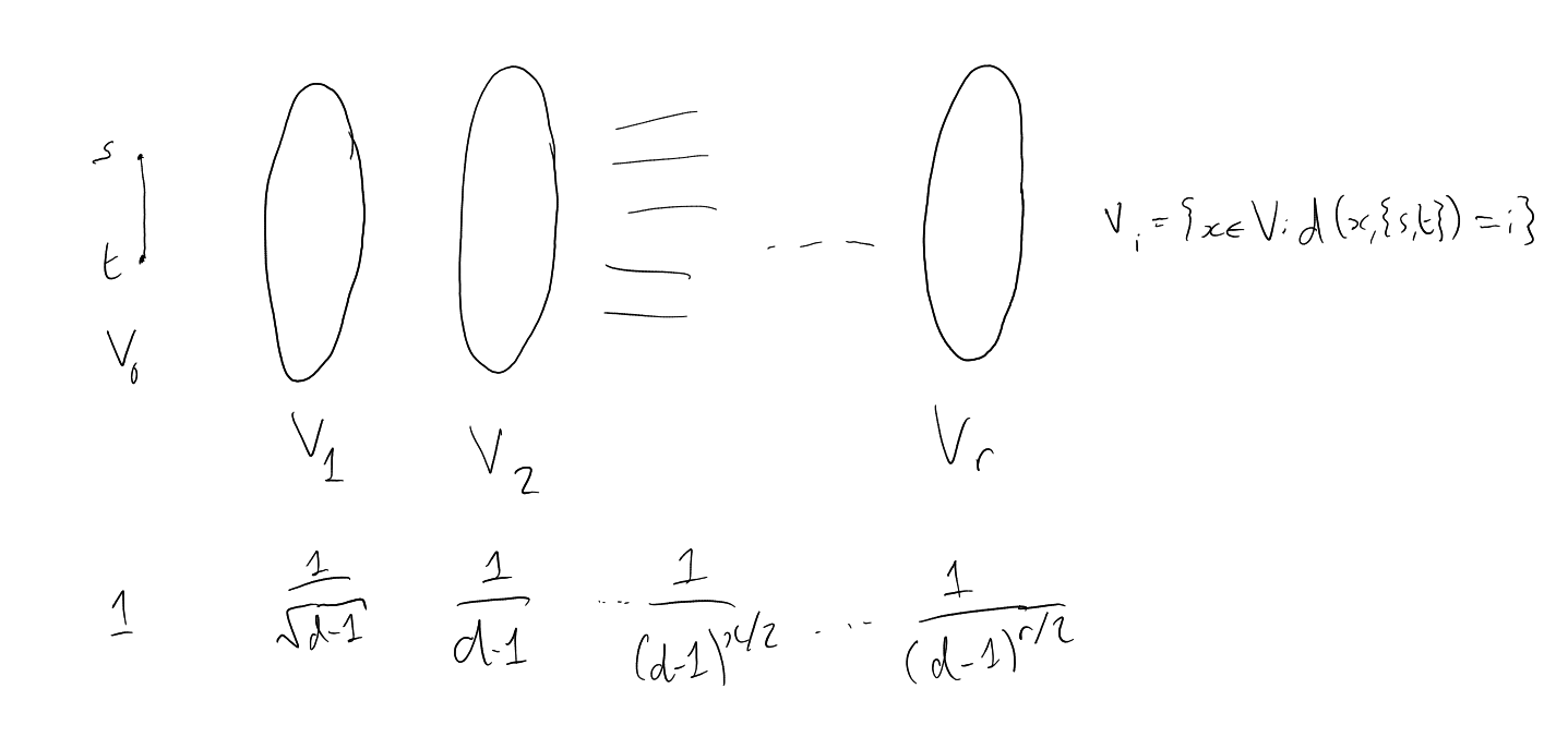
Proof 1. Pick edge st, pick r ∈ ℤ≥0.

PIC

φ : V → ℝ,

φ(x) = { (d − 1)−i∕2 if x ∈ V i, i ≤ r 0 if x ∈ V i, i > r
q L (φ) = ⟨φ,Lφ⟩ ⟨φ,φ⟩ ⟨φ,φ⟩ = ∑ i=0r |V i| (d − 1)i.

⟨φ,Lφ⟩ = ∑ x∼y(φ(x) − φ(y))2 = ∑ i=0r−1e(V i,V i+1) ( 1 (d − 1)i∕2 − 1 (d − 1)(i+1)∕2 ) 2 + e(V r,V r+1) (d − 1)r = ∑ i=0r−1e(V i,V i+1) (d − 1)i (1 − 1 d − 1 )2 + e(V r,V r+1) (d − 1)r e(V i,V i+1) ≤ (d − 1)|V i|. ⟨φ,Lφ⟩ ≤∑ i=0r−1 |V i| (d − 1)i( d − 1 − 1)2 + |V r| (d − 1)r(d − 1) ( d − 1 − 1)2 = (d − 1) − 2 d − 1 + 1 = d − 2 d − 1 ⟨φ,Lφ⟩ ≤ (d − 2 d − 1)∑ i=0r−1 |V i| (d − 1)i + (d − 1) |V r| (d − 1)r |V r| ≤ (d − 1)|V r−1|≤⋯ ≤ (d − 1)r−i|V i| ⟹ |V r| (d − 1)r ≤ 1 r∑ i=0r |V i| (d − 1)i ⟨φ,Lφ⟩ ≤ (d − 2 d − 1)∑ i=0r |V i| (d − 1)i + (2 d − 1) |V r| (d − 1)r ≤ (d − 2 d − 1 + 2 d − 1 − 1 r + 1 )⟨φ,φ⟩ ⟹λ2(L) = min ⁡ dim⁡ ⁡ W=2 max ⁡ f∈W f≠0 ⟨f,Lf⟩ ⟨f,f⟩

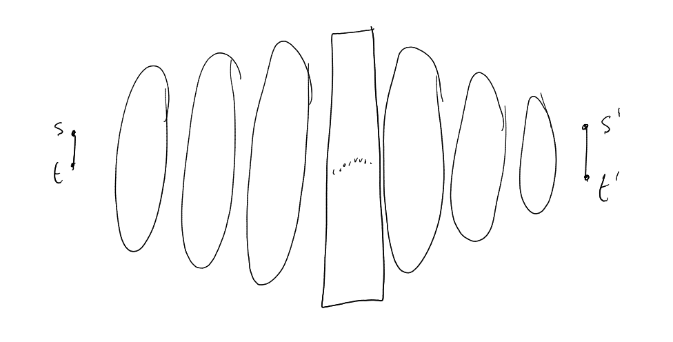
Suppose G has 2 deges at distance > 2r + 2.

PIC

f, f′ as above. ⟨f,f′⟩ = 0.

Q L (αf + βf′) = Q L(αf) + QL(βf′).

Let W = span ⁡ {f,f′}.

λ2(L) ≤ max ⁡ (α,β)≠(0,0) QL (αf + βf′) ∥αf + βf′∥ ≤ α2QL(f) + β2QL(f′) α2∥f∥ + β2∥f′∥ ≤ d − 2 d − 1 + 2 d − 1 − 1 r + 1 □

Corollary 4.10. For all d, there are finitely many (n,d,λ)-graphs with λ < 2 d − 1.

r = clog⁡n.

λn−1(AG) ≥ 2 d − 1 − Od ( 1 log⁡n ).

For Alon-Boppana:

Proof 2. Tr ⁡ A2k = ∑ ⁡ xA2k(x,x). Note that

#{closed walks of length 2k in G starting from x}.

is at least

#{closed walks of length 2k in ∏ d starting from 0}

(∏ ⁡ d is an infinite d-regular tree). The latter is at least

(d − 1)k 1 k + 1 2k k ≈ (2 d − 1)2k+o(1)22k.
≤∑ i=1nλ i2k ≤ d2k + (n − 1)λ2k.

Exercise: finish details. □

min ⁡ {|λ1(A)|λn−1(A)}≥⋯

4.1 One-sided expanders

Goal is to find: Gn graphs with n vertices, d-regular such that λn−1(AG) ≤ λ < d.

Reminder: (Friedman) If G ∼ Gn,d uniform random d-regular graph then

ℙ(Gn is (n,d,2 d − 1 + 𝜀)-graph) → 1.
Φ (Gn) ≥ λ2(L~G) 2 = λ2(LG) 2d = (d − λn−1(AG)) 2d ≥ 1 2 −𝜀 2 > 0.

Theorem 4.11. Assuming that:

  • d = 2l large enough

Then there is 𝜀 = 𝜀d > 0 such that there are d-regular graphs (or multi-graphs) Gn on n vertices with Φ(Gn) ≥ 𝜀 for all sufficiently large n.

Graphs Gn are as follows:

Lemma 4.12. There is c = cd > 0 such that

ℙ(Gn is d-regular, i.e. Gn is simple) ≥ c − o(1).

Lemma 4.13. If Gn is d-regular, then there exists 𝜀 = 𝜀d > 0 such that

ℙ(Φ(Gn) < 𝜀) → 0.

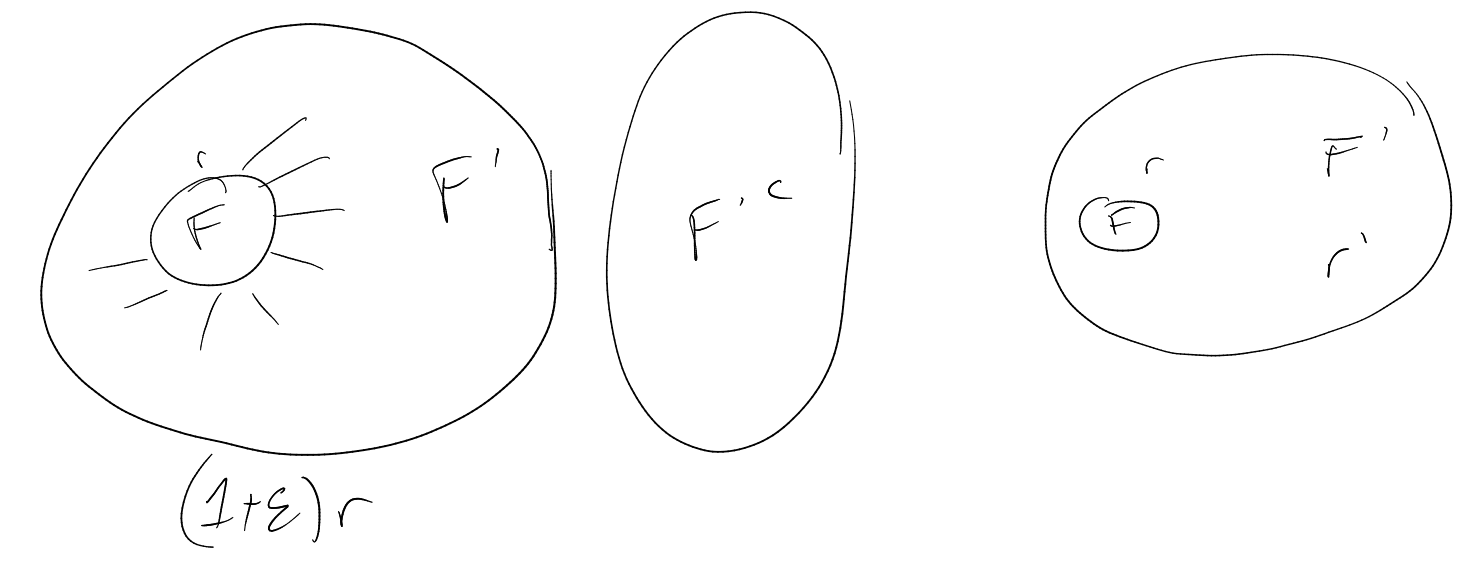
Proof. If Φ(Gn) < 𝜀 then there exists F ⊆ [n], r = |F|≤ n 2 , there exists F′, F ⊆ F′ and e(F,F′) = d|F| and |F′| = r + r′, r′ = ⌊𝜀r⌋.

PIC

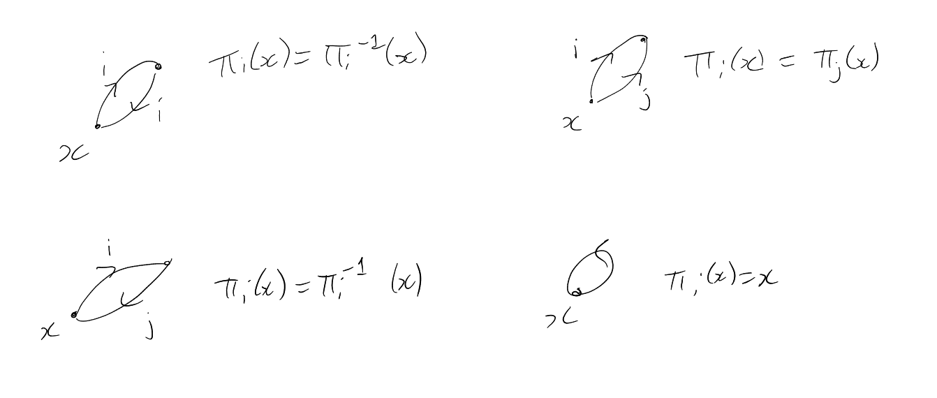
ℙ(Φ(Gn) < 𝜀) < ∑ 1≤r≤n 2 ∑ F⊆F′⊆[n] |F|=r |F′|=r+r′ ℙ(πi(F) ⊆ F′ for all i ∈ [l]).

ℙ(π1(F) ⊆ F′) = r+r′ r n r .

ℙ ≤∑ 1≤r≤n 2 n! r!r′!(n − r − r′)! ( r+r′ r n r ) l.

Fact 1: a k b k ≤ (a b ) k if a ≤ b.

Proof: It is equivalent to

ba ⋅ b(a − 1)⋯b(a − k + 1) ≤ ab ⋅ a(b − 1)⋯a(b − k + 1).

Compare the product term by term.

Fact 2: n! ≥ (n e ) n. Proof:

en = ∑ k≥0 nk k! ≥ nn n! .

Using these:

n! r!r′!(n − r − r′)! ≤ nr+r′ r!r′! = nr+r′ (r + r′)! r + r′ r ≤ (2e)r+r′ ( n e + e′)r+r′ .

So

ℙ ≤∑ 1≤r≤n 2 (2e)r+r′ ( n r + r′)r+r′ ( r + r′ n )lr ≤∑ 1≤r≤n 2 (2e)2r ((1 + 𝜀)r n )r(l−1−𝜀)

Decompose as ∑ ⁡ 1≤r≤n∕2 = ∑ 1≤r≤K + ∑ K<r≤n∕2 = S1 + S2. Choose 𝜀 > 0 small so that γ = 1+𝜀 2 is small. Choose l large so that γl−1−𝜀 < 1 2(2e)2 .

S2 ≤∑ K<r≤n 2 (2e)2r ((1 + 𝜀) 2 )r(l−1−𝜀) ≤∑ K<r≤n 2 ( 1 2 )r ≤ 1 2K

Now S1.

S1 ≤∑ 1≤r≤K(2e)2r ((1 + 𝜀)r n )r(l−1−𝜀) ≤ (2K n )l−2 ∑ 1≤r≤K(2e)2r ≤ cK (K n )l

Now let K = log⁡log⁡log⁡n, so this is ≤ O((log⁡log⁡n)n−l(log⁡log⁡log⁡n)l) → 0. Also, S1 ≤ 1 2K term goes to 0. □

For the lemma about ℙ(d-regular) ≥ c − o(1):

PIC

These are the bad things. Use Bonferroni inequalities (the partial sum of inclusion exclusion principle inequalities).

(n,d,λ)-graph

n: number of vertices, d-regular, λk(A) ∈ [−λ,λ], k≠n.

Ramanujan graph: (n,d,2 d − 1)-graph.

Alon-Boppana: For every 𝜀 > 0 fixed d ≥ 3, there are finitely many (n,d,2 d − 1 − 𝜀)-graphs.

Bipartite: (n,d,λ)-graph, n vertices, d-regular, λk(A) ∈ [−λ,λ] for k≠n,1.

Theorem 4.14 (Lubotsky-Phillips-Sanak / Margoulis). Assuming that:

  • p prime

  • d = p + 1

  • n arbitrarily large

Then there exists a (n,d,2 d − 1)-graph.

Goal:

Theorem 4.15 (Marcus, Spielman, Srivastava). Assuming that:

  • d ≥ 3

Then there are (n,d,2 d − 1)-bipartite graphs for arbitrarily large n.

Strategy: Bilu and Linial. Lifts of graphs:

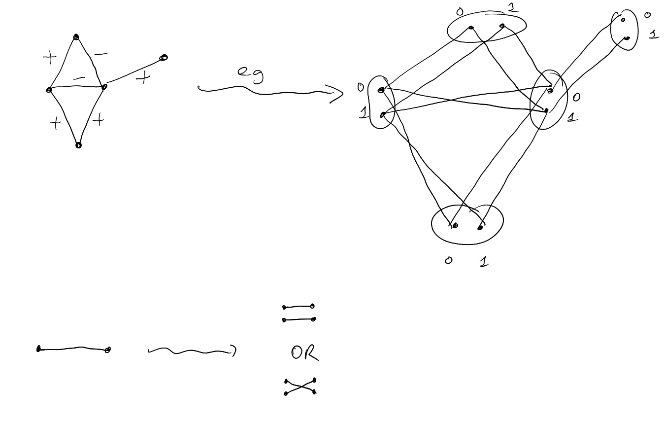
Definition 4.16 (2-lift). A 2-lift of a graph G = (V,E) is a graph Ĝ = (V ^,Ê) with

  • x ∈ V ⟹ x0,x1 ∈V ^.

  • xy ∈ E ⟹ either x0y0,x1y1 ∈Ê or x0y1,x1y0 ∈Ê.

(and no other vertices or edges).

PIC

Definition 4.17 (Signing). S : V × V → ℝ is a signing of G if

S(x,y) = { ±1 if A(x,y) = 1 0 if A(x,y) = 0

and S(x,y) = S(y,x) (symmetric). So can think of S as a function E →{±1}.

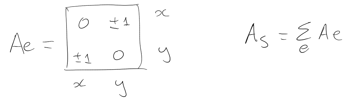
AS+(x,y) = A(x,y)𝟙S(x,y) = 1. AS−(x,y) = A(x,y)𝟙S(x,y) = −1. Have A = AS+ + AS−, S = AS+ − AS−.

Lemma 4.18. The eigenvalues of Ĝ are the eigenvalues of AG (old) together with the eigenvalues of S (new).

Proof.

A ĜS = ( AS+ ASS− AS− ASS+ )

Let Aφ = λφ. Then

A ĜS ( φ φ ) = ( AS+φ + AS−φ AS−φ + AS+φ ) = ( Aφ Aφ ) = ( λφ λφ ) = λ ( φ φ ).

Let Sη = μη. Now

A ĜS ( η −η ) = ( AS+η − AS−η AS−η − AS+η ) = ( Sη −Sη ) = ( μη −μη ) = μ ( η −η ).□

Conjecture 4.19 (Bilu, Linial). If G is d-regular, then there exists a signing S : E(G) →{±1} whose eigenvalues are in [−2 d − 1,2 d − 1].

Theorem 4.20 (Bilu, Linial). Can find signings S with eigenvalues λ satisfying |λ| = O( d(log⁡d)3).

Theorem 4.21 (Marcusm, Spielman, Srivastava). Assuming that:

  • G is a d-regular graph

Then there exists a signing with eigenvalues λ with λ ≤ 2 d − 1.

Theorem 4.21 implies Theorem 4.15.

Notation. For π ∈ Sym ⁡ (X), let |π| be the number of inversions.

Theorem 4.21: S ∼ Unif ⁡ ({±1}E(G)).

𝔼S det ⁡ (xI − S) = 𝔼S (∑ π∈Sym ⁡ (X)(−1)|π|∏ y∈V (xI − S)(y,π(y))) = ∑ k=0nxn−k(−1)k ∑ T⊆V |T|=k ∑ π∈Sym ⁡ (T)𝔼S ((−1)|π|∏ y∈T(xI − S)(y,π(y)))

For xy ∈ E: 𝔼S(x,y)2k+1 = 0, 𝔼S(x,y)2k = 1.

PIC

= ∑ k=0 k even nxn−k(−1)k ∑ M matching of size  ≤ k 2 (−1)k∕2… = ∑ k≥0xn−2k(−1)kM k(G) = μG(x) where Mk(G) is the number of matchings of size k in G.

μG(x) is the matching polynomial of G.

Heilman-Lieb-Godsil:

Last time, when working on det ⁡ (xI − As), we showed:

Theorem 4.22 (Godsil-Gutman, 80s).

𝔼S∼{±1}det ⁡ (xI − As) = μG(x),

where

μG(x) = ∑ k≥0xn−2k(−1)km k(G),

where mk(G) is the number of matchings in G with k edges.

Fact: μG(x) is real rooted.

Theorem 4.23 (Heilman-Lieb, 72). Assuming that:

  • G is d-regular

Then
maxroot ⁡ μG(x) ≤ 2 d − 1.

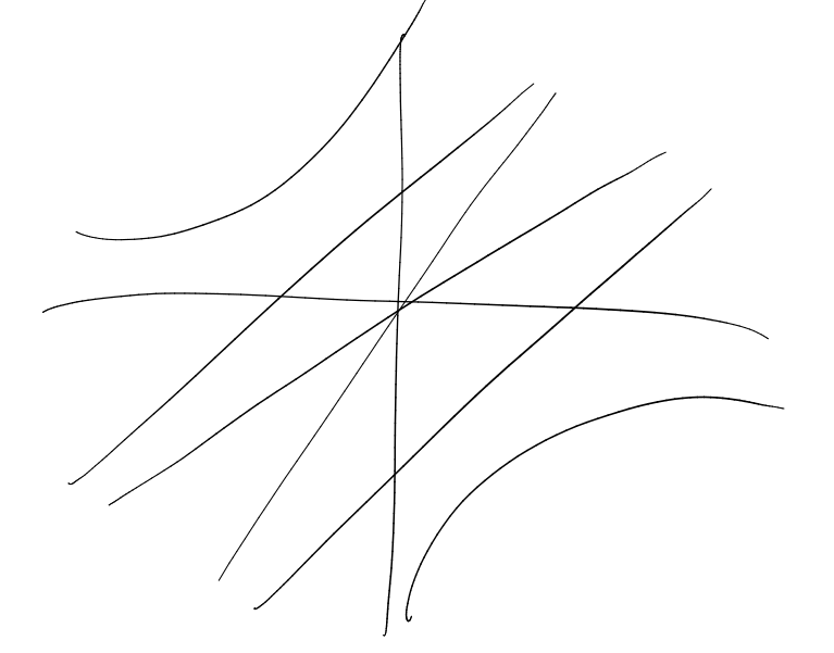
If only we could say that maxroot ⁡ 𝔼S det ⁡ (xI − As) is an average of maxroot ⁡ det ⁡ (xI − Ah), h ∈{±1}E. Hopelessly false:

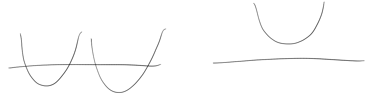
PIC

Definition 4.24 (Interlacing). Let f be a real rooted polynomial of degree n with roots α1,…,αn and g a real rooted polynomial of degree n − 1 with roots β1,…,βn−1. We say g interlaces f if

α1 ≤ β1 ≤ α2 ≤⋯ ≤ βn−2 ≤ αn−1 ≤ βn−1 ≤ αn.

PIC

Example. If f is real rooted, then so is f′, and also f′ interlaces f.

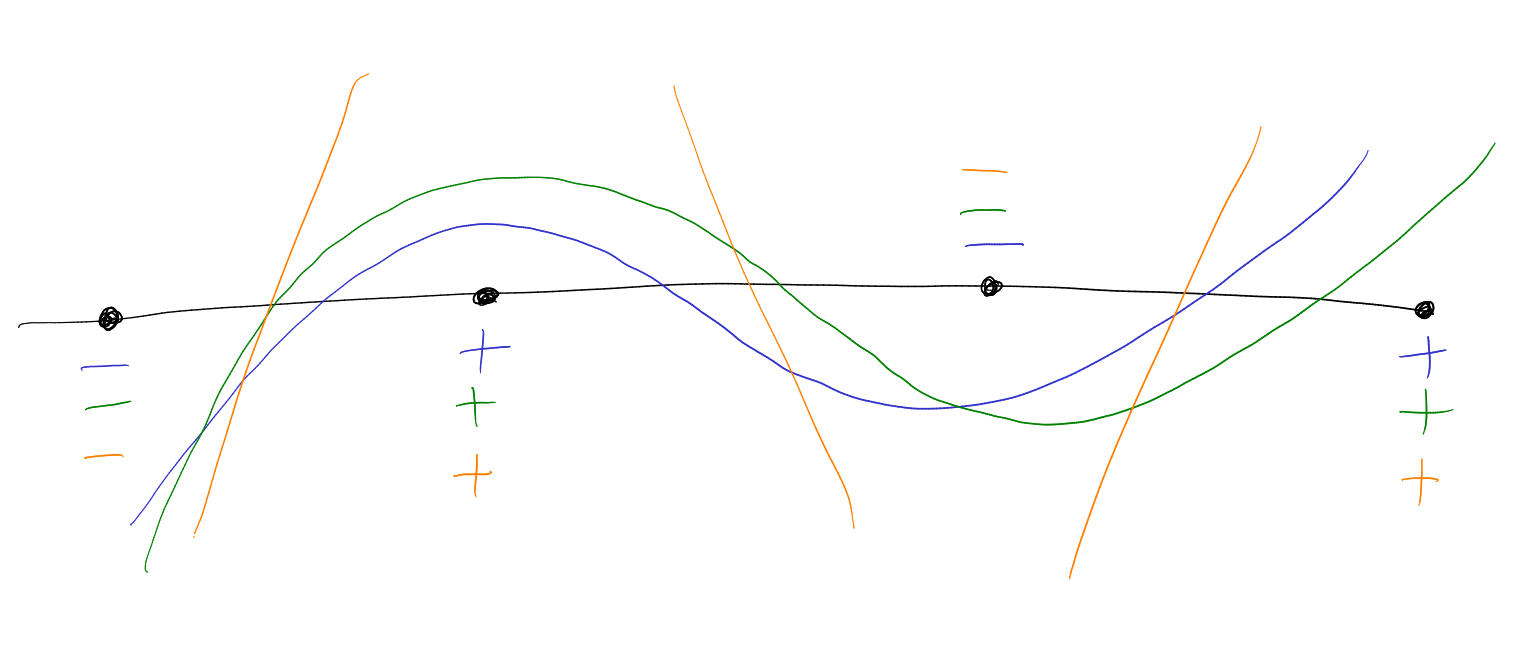
Definition 4.25 (Common interlacement). We say that real rooted polynomials f, g of degree n have a common interlacement if there is a polynomial h of degree n + 1 such that f and g both interlace h. In other words, if the roots of f and g are α1 ≤⋯αn and β1 ≤⋯ ≤ βn respectively, then they have a common interlacement if and only if there are some γ0 ≤⋯ ≤ γn such that

γ0 ≤ α1,β1 ≤ γ1 ≤ α2,β2 ≤ γ2 ≤⋯ ≤ γn−1 ≤ αn,βn ≤ γn.

Theorem 4.26 (Fell 80). Assuming that:

  • f, g are real rooted

  • both degree n, monic

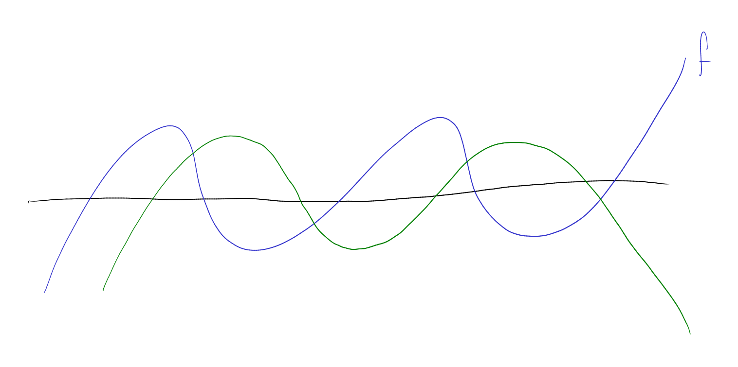
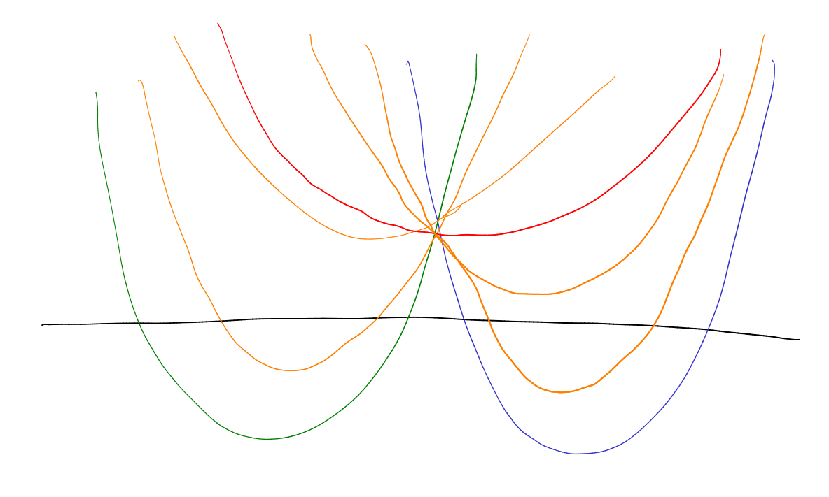
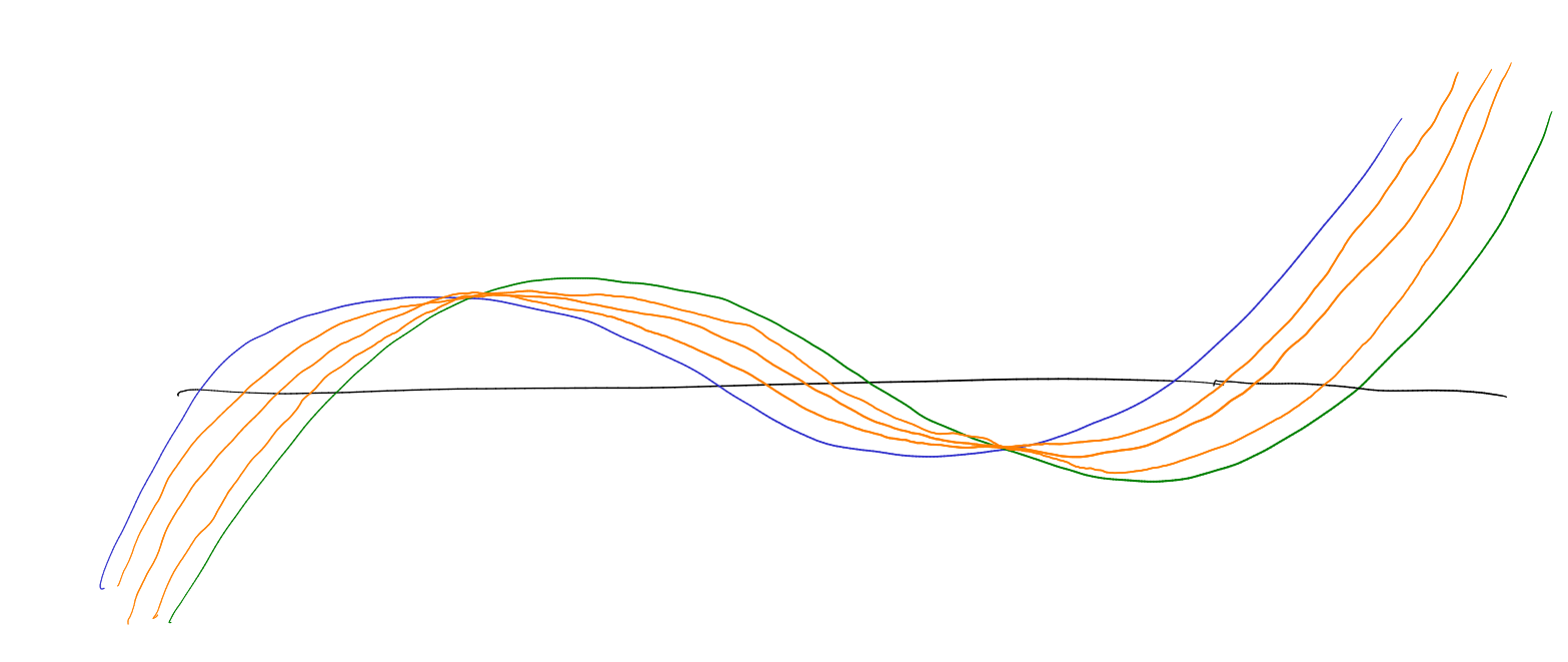
Then f and g have a common interlacing if and only if every convex combination of f and g are real rooted.

PIC

PIC

Proof. Assume f and g without repeated or common roots (general case requires more work and details checking).

Corollary 4.27. Assuming that:

  • f, g are real rooted of degree n

  • have a common interlacing

Then for all t ∈ [0,1]
min ⁡ {maxroot ⁡ (f),maxroot ⁡ (g)}≤ maxroot ⁡ (tf(x) + (1 − t)g(x)).

Approach to Theorem 4.21:

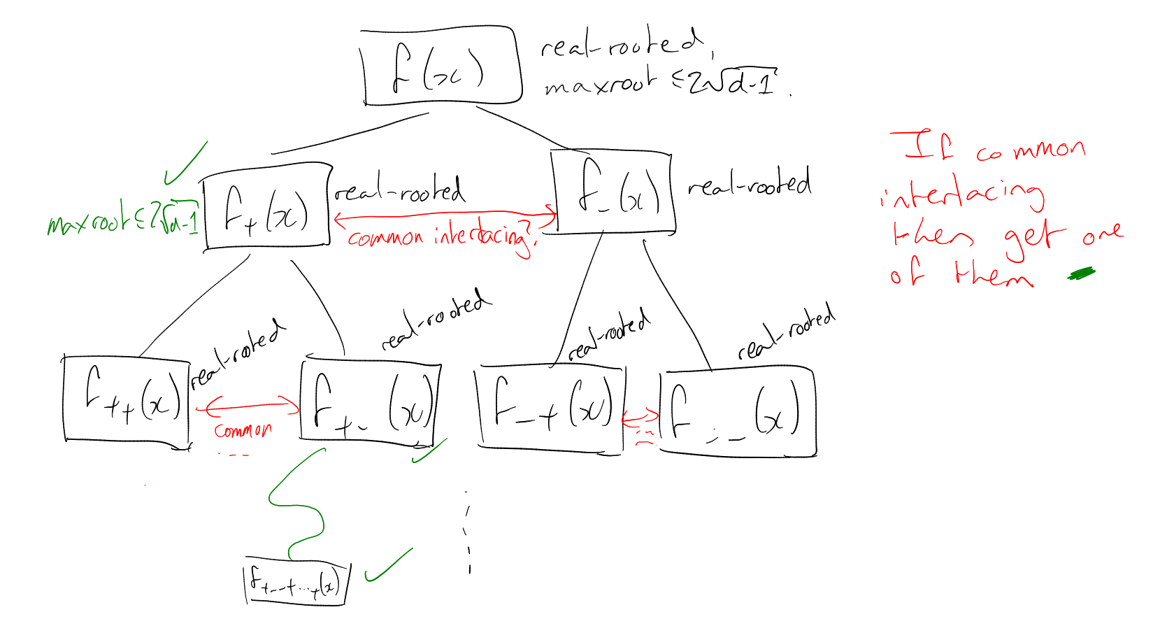
f(x) = 𝔼S∈{±1}E det ⁡ (xI − As), |E| = m. For h1,…,hk ∈{±1} = {+,−}, then

fh1,…,hk(x) = 𝔼sk+1,…,sm∈{±1}(det ⁡ (xI − As)|s1 = h1,… ⁡ ,sk = hk).

“Method of interlacing families of polynomials”

PIC

Theorem 4.28 (Marcus, Spielman, Srivastava (real rooted)). For every ρ1,…,ρm ∈ [−1,1] the following polynomial is real rooted

χρ1,…,ρm(x) = ∑ S∈{±1}m det ⁡ (xI − As)∏ J:sJ=1 ( 1 + ρJ 2 )∏ J:SJ=−1 ( 1 − ρJ 2 ).

Theorem 4.28 implies Theorem 4.21:

fh1,…,hk(x) = χh1,…,hk,0,0,…,0(x).
μG(x) = χ0,…,0(x).
tfh1,…,hk,1(x) + (1 − t)fh1,…,hk,−1(x) = χh1,…,hk,2t−1,0,…,0(x).

Theorem 4.29 (Marcus, Spielman, Srivastava (matrix)). Assuming that:

  • r1,…,rm ∈ ℝn are independent random vectors, whose support has ≤ 2 points

Then
𝔼 det ⁡ (xI −∑ j=1mr jrj⊤ ⁡)

is real rooted.

Theorem 4.29 implies Theorem 4.28:

χρ1,…,ρm(x) is

𝔼 det ⁡ (xI − As).

PIC

𝔼 det ⁡ (xI − As) is real rooted if and only if 𝔼 det ⁡ ((x + d)I − As) is real rooted. This equals

𝔼 det ⁡ (xI + (dI − As)).

Note

dI − AS = ∑ x∼y(ex + S(x,y)ey)(ex + S(x,y)ey)⊤ ⁡.

Done.

Definition 4.30 (Real stable). A polynomial p(z1,…,zn) ∈ ℝ[z1,…,zn] is real stable if p(z1,…,zn)≠0 for all (z1,…,zn) ∈Hn, H = {z ∈ ℂ|Im ⁡ z > 0}.

Notice that for a single variable, p(z) is real stable if and only if real rooted.

Example. 1 − z1z2.

Proposition 4.31 (Stable iff real rooted). p(z1,…,zn) is real stable if and only if for all ℝ≥0n, b ∈ ℝn, the polynomial t↦p(at + b) is real rooted.

Proof.

Proposition 4.32 (Stability of real stable). Assuming that:

  • p(z1,…,zn) is real stable

Then the following are also:
  • p(zσ(1),…,zσ(n)), σ ∈ Sn.

  • p(az1,z2,…,zn), a ∈ ℝ≥0.

  • p(z2,z2,z3,…,zn).

  • p(c,z2,…,zn), c ∈H ∪ ℝ.

  • z1d1p (−1 z1 ,z2,…,zn).

  • ∂z1p(z1,…,zn).

  • MAP ⁡ (p(z1,… ⁡ ,zn)). MAP ⁡ (z1z2 + z2z32 + 2z1z4 + z2z32) = z1z2 + 2z1z4.

  • If p,q are real stable, then so is pq.

Proposition 4.33 (Mother of all stable polynomials). Assuming that:

  • B ∈ ℝd×d symmetric matrix

  • A1,…,Am ∈ ℝd×d positive semi definite

Then det ⁡ (B + z1A1 + ⋯ + znAn) is real stable.

Proof. Let a ∈ ℝ≥0n, b ∈ ℝn. Assume positive definite instead of positive semi definite.

det ⁡ (B + ∑ j=1n(a jt + bj)Aj) = det ⁡ ((∑ j=1na jAj)⏟ =:At + (∑ j=1nb jAj + B)⏟=:C)

A is positive definite, and C is symmetric. So

= det ⁡ (At + C) = det ⁡ (A1 2 (tI + A−1 2 CA−1 2 )A1 2 ) = det ⁡ Adet ⁡ (tI + A−1 2 CA−1 2 )

The roots are eigenvalues of a real symmetric matrix, hence real. □

Proof of Theorem 4.29. Say rj equals rj+ with probability pj+, and equals rj− with probability pj−. We will use Cauchy Binet:

det ⁡ (AB) = ∑ det ⁡ (AS×[n])det ⁡ (B[n]×C)TODO

p(z1,…,zn) = 𝔼 det ⁡ (∑ j=1nz jrjrj⊤ ⁡) = 𝔼 ∑ S⊆[m] |S|=n det ⁡ (∑ j∈Szjrjrj⊤ ⁡) = 𝔼 ∑ S⊆[m] |S|=n (∏ j∈Szj) det ⁡ (∑ j∈Srjrj⊤ ⁡)
det ⁡ (𝔼 ∑ j=1nz jrjrj⊤ ⁡) = det ⁡ (∑ j=1nz j𝔼rjrj⊤ ⁡)

is real stable since 𝔼rjrj⊤ ⁡≥ 0 is a covariance matrix.

= det ⁡ (∑ j=1mz j(pj+r j+(r j+)⊤ ⁡ + p j−r j−(r j−)⊤ ⁡)) = ∑ S⊆[m] |S|=n (∏ j∈Szj) ∑ n∈{±1}S det ⁡ (pjh(j)r jh(j)(r jh(j))⊤ ⁡) + “terms with squares”

So the earlier thing is real stable. So

𝔼 det ⁡ (∑ j=1mz jrjrj⊤ ⁡)

is real stable. So

𝔼 det ⁡ (∑ j=1mz jrjrj⊤ ⁡ + ∑ j=1mx jejej⊤ ⁡)

is real stable. Take zj = −1, xj = x. Then

𝔼 det ⁡ (xI −∑ j=1mr jrj⊤ ⁡)

is real stable. □

Theorem 4.34 (Godsil). Assuming that:

  • G is d-regular

  • λ1 ≤⋯ ≤ λn are the roots of μG(x)

Then
∑ k=1nλ kl = ∑ aWal(G),

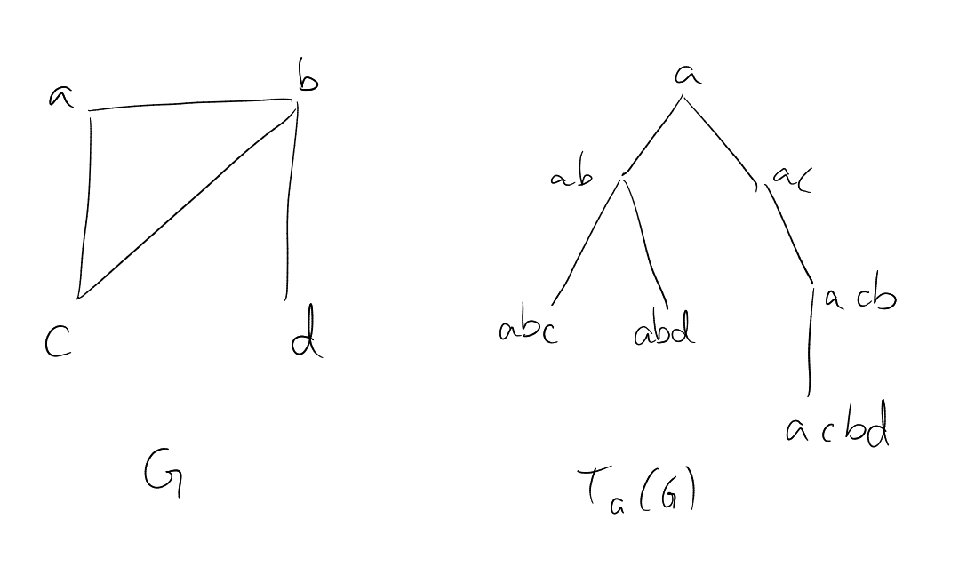
where Wal(G) is the number of closed walks of length l from a in the path tree Ta(G) of G.

Definition 4.35 (Path tree). Example: Ta(G)

PIC

Proof of ?? implies Theorem 4.23. Wal(G) ≤ Wal(∏ ⁡ d) ≤ (2 d − 1 + ol(1))l.

λnl ≤∑ ⁡ λkl = ∑ aWal(G) ≤ n(2 d − 1 + ol(1))l.

λn ≤ n1 l (2 d − 1 + ol(1)).

Take l →∞. □

Proof of ??. μG′(x) = ∑ ⁡ aμG−a(x) Hence

∑ a ∑ k≥0xn−1−2k(−1)km k(G − a) = ∑ k≥0(n − 2k)xn−1−2k(−1)km k(G) = μG′(x)

μG(x) = xμG−a(x) −∑ b∼aμG−a−b(x) mk(G) = mk(G − a) + ∑ b∼amk−1(G − a − b) xn−2k(−1)km k(G) = x ⋅ xn−1−2k(−1)km k(G − a) −∑ b∼axn−2−2(k−1)(−1)k−1m k−1(G − a − b) ∑ a μG−a(x) μG(x) = μG′(x) μG(x) = ∑ j=1n 1 x − λj = 1 x∑ j=1n 1 1 −λj x = 1 x∑ j=1n ∑ l≥0 λjl xl = 1 x∑ l≥0 ∑ jλjl xl Claim: μG−a(x) μG(x) = 1 x ∑ ⁡ l≥0Wal(G) xl . μG−a(x) μG(x) = μG−a(x) xμG−a(x) −∑ b∼aμG−a−b(x) = 1 x 1 1 −1 x ∑ b∼aμG−a−b(x) μG−a(x) = 1 x ⋅∑ k≥0 ( 1 x∑ b∼a μG−a−b(x) μG−a(x) )k = 1 x∑ k≥0 1 xk (∑ b∼a 1 x∑ l≥0 Wbl(G − a) xl ) k = 1 x∑ k≥0 1 x2k (∑ b1∼a ∑ l1≥0 WGl1(G − a) xl 1 ) ⋯ (∑ bk∼a ∑ lk≥0 Wbklk(G − a) xl k ) = 1 x∑ l≥0 Wal(G) xl

Why? A tree-like walk in Wal(G) that visits a exactly k times is determined by:

□

˙

Index

(d,𝜀)-expander

𝜀-approximation

Hermitian

(n,d,λ)-graph